If you’ve dabbled in data visualization, there’s a good chance you’ve
encountered the colormap viridis, which was created for matplotlib in
~2015.
You may also know about some of the considerations went into the colormap’s design, chiefly perceptual uniformity: equally distant colors on the colormap should “look equally different” to humans.
I won’t discuss color theory much here; the talk introducing viridis (below) is quite good, and there are many other resources online, such as Jamie Wong’s From Hexcodes to Eyeballs or Bartosz Ciechanowski’s Color Spaces.
Instead, I nerd-sniped myself with a different question: How is viridis, specifically, defined?
This seems like it should be easy to answer. Just go into matplotlib and find the source code for viridis, right? Unfortunately, that source code is just a list of 256 RGB triples along which colors are interpolated. This makes sense for efficiency and even portability because (as we’ll see) the formula for producing viridis is incredibly complicated, but it isn’t a very satisfying answer. How did those triples originally come to be?
The color space
The first ingredient of viridis is the uniform color
space it uses, CIECAM02-UCS, which parametrizes colors by the three
variables \(J'\), \(a'\), and \(b'\). CIECAM02-UCS is built on top of
CIECAM02, a color
appearance model published in 2002.
Actually, CIECAM02-UCS and CIECAM02 don’t provide a single mapping of colors to their spaces. You have to set something like eight other parameters:
- whitepoint in the XYZ color space \(X_w, Y_w, Z_w\)
- background luminance \(Y_b\)
- luminance of the adapting field \(L_A\)
- degree of adaptation \(F\)
- impact of surrounding \(c\)
- chromatic induction factor \(N_c\)
Given those parameters, CIECAM02 provides a mapping between colors and seven “appearance correlates” \((J, C, h, Q, M, s, H)\). CIECAM02-UCS then defines a mapping between \((J, M, h)\) and \((J', a', b')\). I’m not going to explain what all these variables mean (not least because I don’t understand them), but I hope that knowledge of their existence helps contextualize how complicated the model we’re working with.
It happens that viridis was originally generated with a
buggily
parametrized of CIECAM02-UCS where \(L_A\) was 125× too large, i.e. the viewing
conditions are 125× lighter than the default. However, it turns out that
this only marginally affects the perceptual uniformity, so nobody has
bothered to fix it.


The code to convert between all these colorspaces is also super
complicated. The colorspacious library internally has a graph
of colorspaces it knows how to convert between, and literally uses a
breadth-first search to find paths between pairs of colorspaces it’s
asked to convert between. The conversion between sRGB and CIECAM02-UCS
has four edges: sRGB ↔︎ XYZ100 ↔︎ CIECAM02 ↔︎ CIECAM02-UCS.
Aside: Other color appearance models
There are far more color appearance models than I expected. CIELAB was the perceptually uniform color space I was familiar with, but it was published in 1976 and is not that good (at being perceptually uniform) by today’s standards. CIECAM02 and its UCS have a successor from 2016, CAM16 and CAM16-UCS, but they don’t seem that popular, I assume because they’re even more complicated than CAM02.
I think the most popular “modern” color space is Oklab, created by Björn Ottosson in 2020, which is super simple — a cube root sandwiched by two 3×3 linear transformations — but punches well above its weight, and has decent CSS support in browsers (93% as of time of writing1). Raph Levien has an interactive review that compares it to several other contenders.
The parameters
The second ingredient to viridis is just a bunch of
numbers from “option
d” in the original repo. These are somewhat arbitrary, as they were
produced by a human dragging points around in a custom GUI, which you
can see at 15:55 in the
viridis talk.
parameters = {
    'xp': [22.674387857633945, 11.221508276482126, -14.356589454756971, -47.18817758739222, -34.59001004812521, -6.0516291196352654],
    'yp': [-20.102530541012214, -33.08246073298429, -42.24476439790574, -5.595549738219887, 42.5065445026178, 40.13395157135497],
    'min_JK': 18.8671875,
    'max_JK': 92.5,
}
min_JK and max_JK specify a minimum and
maximum value along the \(J\)-axis,
while xp and yp (somewhat confusingly) specify
six control points for a Bezier curve in the \(ab\)-plane. Then, the colors of viridis are
obtained by linearly interpolating between min_JK and
max_JK and moving along the curve by arc length in the
\(ab\)-plane. Arc length is also just
approximated by splitting the curve into linear segments.
Here is some code that drills somewhat deeply into viscm
and colorspacious to produce viridis:
from viscm.gui import BezierCMapModel
from viscm.bezierbuilder import SingleBezierCurveModel, ControlPointModel
import numpy as np
from colorspacious import (
    CIECAM02Space,
    CIECAM02Surround,
)

xp = [
    22.674387857633945,
    11.221508276482126,
    -14.356589454756971,
    -47.18817758739222,
    -34.59001004812521,
    -6.0516291196352654,
]
yp = [
    -20.102530541012214,
    -33.08246073298429,
    -42.24476439790574,
    -5.595549738219887,
    42.5065445026178,
    40.13395157135497,
]
min_JK = 18.8671875
max_JK = 92.5

buggy_sRGB_viewing_conditions = CIECAM02Space(
    XYZ100_w="D65",
    Y_b=20,
    L_A=(64 / np.pi) * 5,  # bug: should be / 5
    surround=CIECAM02Surround.AVERAGE,
)

buggy_CAM02UCS = {
    "name": "CAM02-UCS",
    "ciecam02_space": buggy_sRGB_viewing_conditions,
}

model = BezierCMapModel(
    bezier_model=SingleBezierCurveModel(
        control_point_model=ControlPointModel(xp=xp, yp=yp), method="Bezier"
    ),
    min_Jp=min_JK,
    max_Jp=max_JK,
    uniform_space=buggy_CAM02UCS,
)

print(model.get_sRGB(256)[0].tolist())
Expanded in gory detail
Still, I wanted to dig deeper, so I manually inlined all the conversion formulae and performed constant folding and cancellation of a few roundtrip things like conversions between radians and degrees, just to see what it would look like:
import math
import numpy as np

xp = [
    22.674387857633945,
    11.221508276482126,
    -14.356589454756971,
    -47.18817758739222,
    -34.59001004812521,
    -6.0516291196352654,
]
yp = [
    -20.102530541012214,
    -33.08246073298429,
    -42.24476439790574,
    -5.595549738219887,
    42.5065445026178,
    40.13395157135497,
]
min_Jp = 18.8671875
max_Jp = 92.5


def bezier(t, p):
    n = len(xp) - 1
    ret = np.zeros_like(t)
    for k, c in enumerate(p):
        ret += math.comb(n, k) * t**k * (1 - t) ** (n - k) * c
    return ret


def get_sRGB(num=256):
    at = np.linspace(0, 1, num)
    grid = np.linspace(0, 1, 1000)

    # Interpolate along arc length:

    arclength_deltas = np.concatenate(
        [np.zeros((1,)), np.hypot(np.diff(bezier(grid, xp)), np.diff(bezier(grid, yp)))]
    )
    arclength = np.cumsum(arclength_deltas)
    arclength /= arclength[-1]
    at_grid = np.interp(at, arclength, grid)

    # Construct the desired Jp, ap, bp args:

    ap, bp = bezier(at_grid, xp), bezier(at_grid, yp)
    Jp = (max_Jp - min_Jp) * at + min_Jp

    # Convert from Jpapbp to sRGB in a bunch of intermingled steps:

    J = -Jp / (0.007 * Jp - 1.7)
    Mp = np.hypot(ap, bp)
    p_2 = 1.2400517785408007 * J**0.7520055720356568 + 0.305
    denom = (
        0.9266715362288499
        * (ap * np.cos(2) - bp * np.sin(2) + 3.8 * Mp)
        * (np.sqrt(J) / (np.exp(0.0228 * Mp) - 1)) ** (10 / 9)
        + 0.47826086956521735 * ap
        + 4.695652173913044 * bp
    )
    RGBprime_a = (
        np.array(
            [
                [460, 451, 288],
                [460, -891, -261],
                [460, -220, -6300],
            ], dtype=float
        ) @
        np.stack([p_2, p_2 * ap / denom, p_2 * bp / denom])
        / 1403
        - 0.1
    )
    RGBprime = (
        np.sign(RGBprime_a)
        * 125.22084473955428
        * ((27.13 * np.abs(RGBprime_a)) / (400 - np.abs(RGBprime_a))) ** (1 / 0.42)
    )
    sRGB_linear = np.array(
        [
            [
                0.05445103258222664,
                -0.045965885248447864,
                0.0016306136373998147,
            ],
            [
                -0.011667849760570772,
                0.023233202975236258,
                -0.0015950261251939332,
            ],
            [
                0.00037596436229076315,
                -0.001981804005149333,
                0.011546891102251636,
            ],
        ]
    ) @ RGBprime
    return np.where(
        sRGB_linear <= 0.0031308,
        sRGB_linear * 12.92,
        1.055 * sRGB_linear ** (1 / 2.4) - 0.055,
    ).T

print(get_sRGB())
Pretty complicated!
Approximating viridis
I wasn’t fully transparent with my intentions at the beginning of this post. The thought beneath the XY problem was, if I wanted to get a viridis-like colorscheme in a new programming language, how little code could I do it with?
After working out the above code, I decided it was easier to
approximate viridis as a black box. There is precedent online: here’s a
shadertoy with a
degree-6 polynomial approximation of viridis and the other
matplotlib colorschemes. It looks like they built on somebody else’s
methodology, with a tweak to minimize maximum error rather than least
squares error. I decided to do a similar thing, but try to minimize
maximum linear RGB distance, approximated using the derivative
of linear RGB at the known colors, so that we can just do linear
programming.
scipy.optimize.linprog
will do the heavy lifting.
After trying a few degrees, I settled on 4 and 7 as good enough points on the tradeoff curve:
import option_d
import numpy as np
import scipy.optimize

viridis = np.array(option_d.cm_data)

for degree in [4, 7]:
    print(f"{degree=}")
    for column in viridis.T:
        # Optimize a length-(degree+2) vector, whose first (degree+1) elements
        # are the coefficients of the polynomial approximation and whose last
        # element is the maximum allowed approximation of linear RGB distance
        # (let's call it "tolerance")

        # We have 512 constraints, two per point in original viridis, that
        # the point differs from the approximation by less than the tolerance.
        # The first 256 constraints check that (approximation - tolerance <= original)
        # The last 256 constraints check that (-approximation - tolerance <= -original)

        constraints = np.zeros((512, degree + 2))
        # Weight the tolerance by the derivative of linear RGB at the known
        # viridis channel value:
        weight = np.where(column < 0.04045, 1/12.92, ((column + 0.055)/1.055)**1.4 / 1.055)
        constraints[:, -1] = -1/np.concatenate([weight, weight])
        # Coefficients for the coefficients:
        constraints[:256, :-1] = np.linspace(0, 1, 256)[:, None] ** np.arange(degree + 1)
        constraints[256:, :-1] = -(np.linspace(0, 1, 256)[:, None] ** np.arange(degree + 1))

        # The constant RHS:
        cbound = np.concatenate([column, -column])

        # We just want to minimize the tolerance:
        minimizer = np.zeros((degree + 2,))
        minimizer[-1] = 1

        # (Note, we might have wanted to add a hard constraint that our
        # polynomial approximation stays within [0, 1], but fortunately it
        # doesn't affect our answer)

        result = scipy.optimize.linprog(minimizer, A_ub=constraints, b_ub=cbound, bounds=(None, None))
        print(result.x[:-1])
Rounded and formatted ready-to-copy code, here are the results:
def degree_four_viridis(t):
    return [
        (((-5.5793*t + 13.5837)*t - 8.5613)*t + 1.3097)*t + 0.2446,
        (((-0.5587*t +  0.7695)*t - 0.5851)*t + 1.2498)*t + 0.0284,
        ((( 0.5341*t -  0.8296)*t - 1.0321)*t + 1.0515)*t + 0.3552,
    ]

def degree_seven_viridis(t):
    return [
        ((((((42.3473*t - 148.6685)*t + 194.9250)*t - 119.0426)*t + 37.8497)*t - 7.2161)*t + 0.5286)*t + 0.2707,
        (((((( 4.8916*t -  12.2295)*t +   9.1748)*t -   1.3875)*t -  0.2732)*t - 0.7410)*t + 1.4669)*t + 0.0041,
        ((((((22.6620*t -  56.3548)*t +  54.0592)*t -  29.8980)*t + 13.5239)*t - 6.0311)*t + 1.8471)*t + 0.3253,
    ]
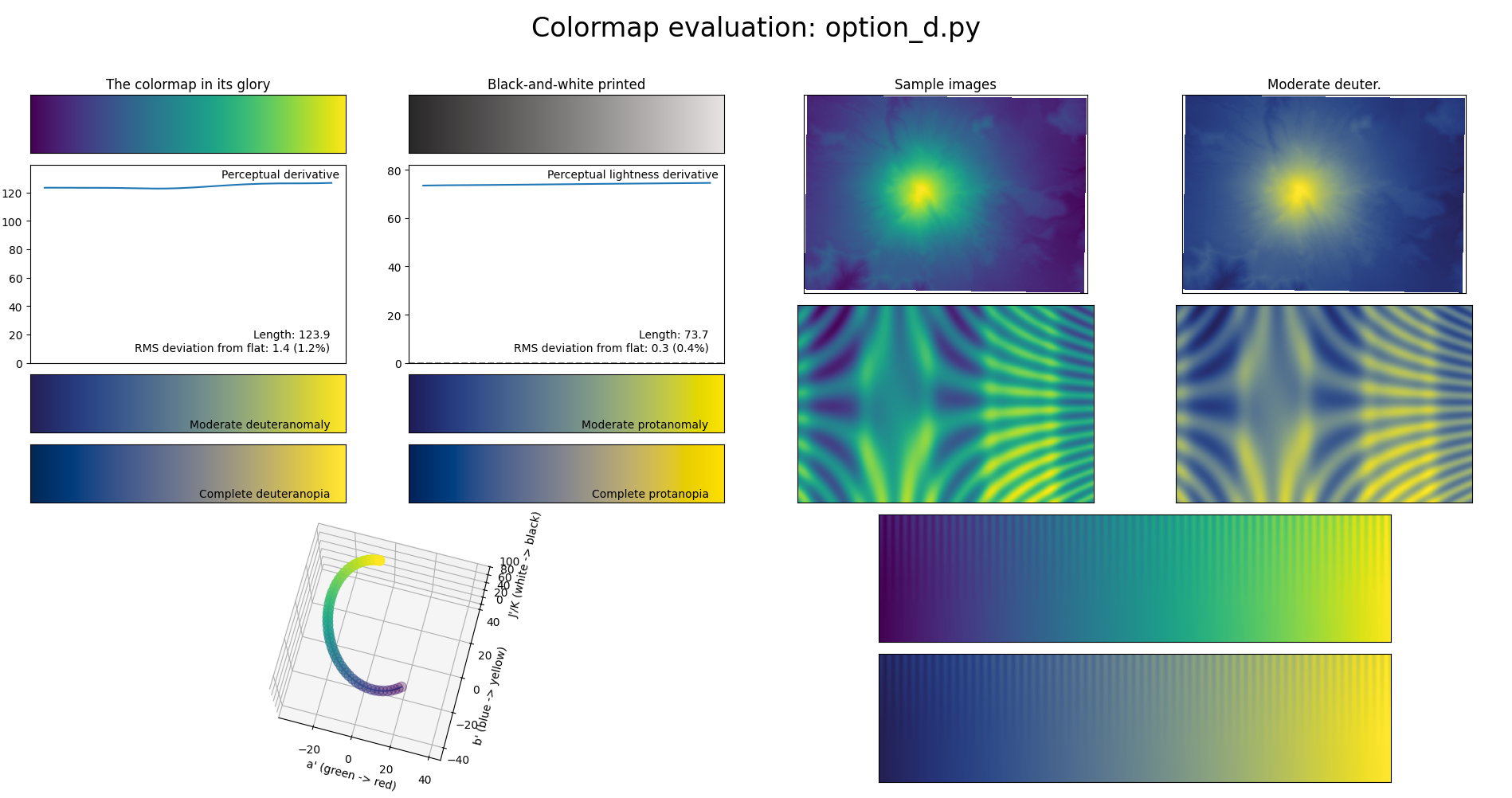
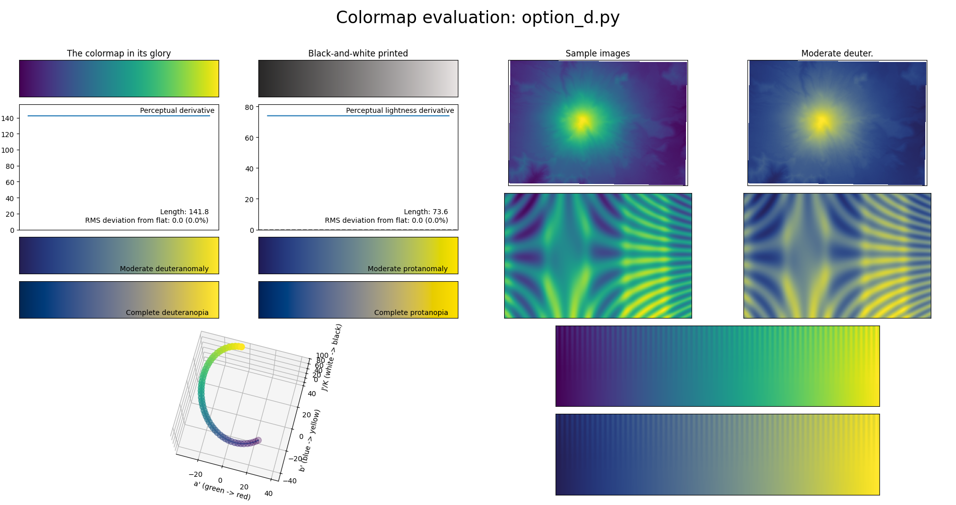
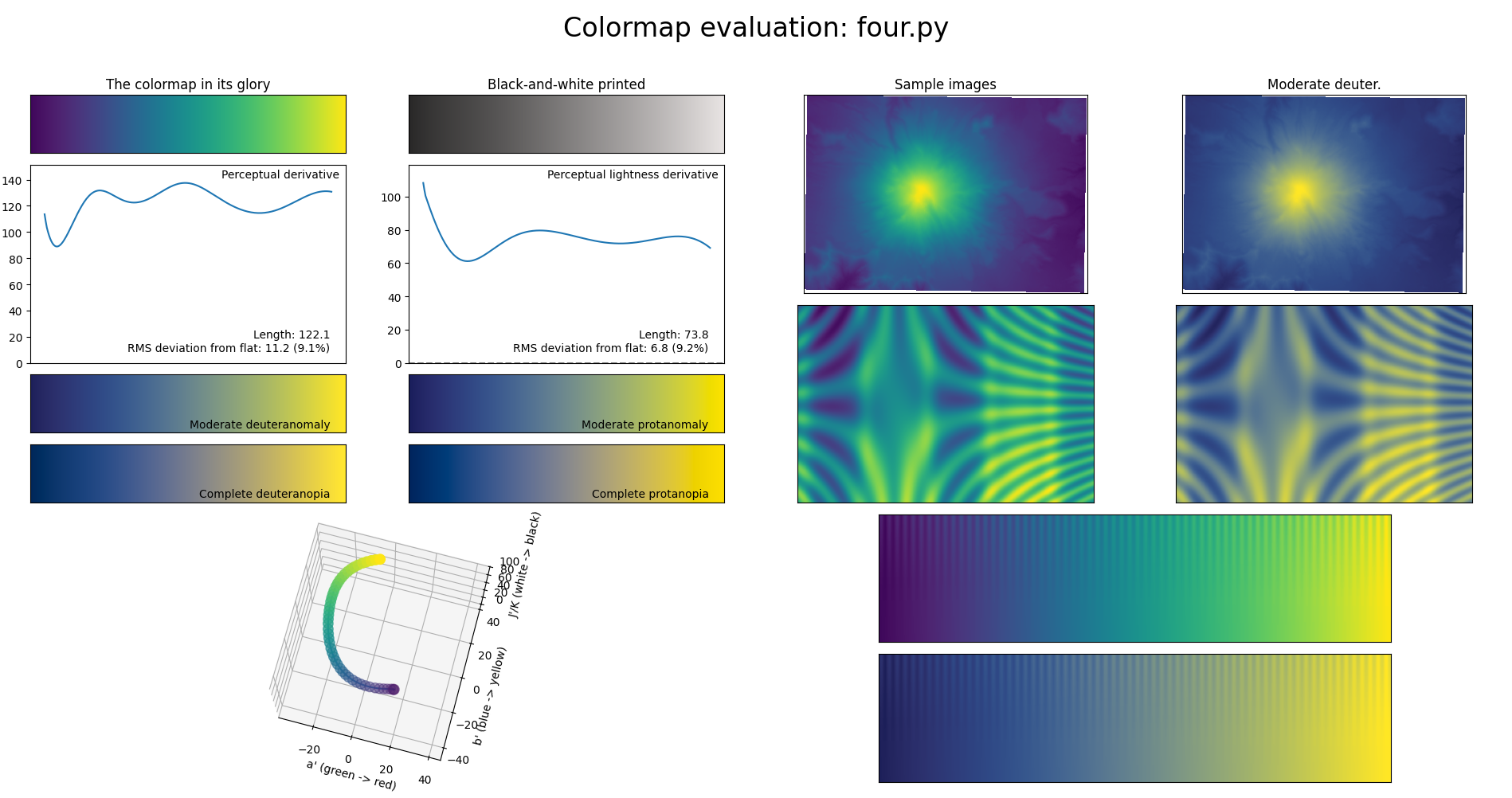
There are three stripes in the above figure: in order, original viridis, the degree-7 approximation, and the degree-4 approximation. I can’t tell the difference between viridis and the degree-4 approximation unless I squint quite a bit, and only on the lower end. I can’t tell the difference between viridis and the degree-7 approximation at all.


Approximating viridis and its desiderata
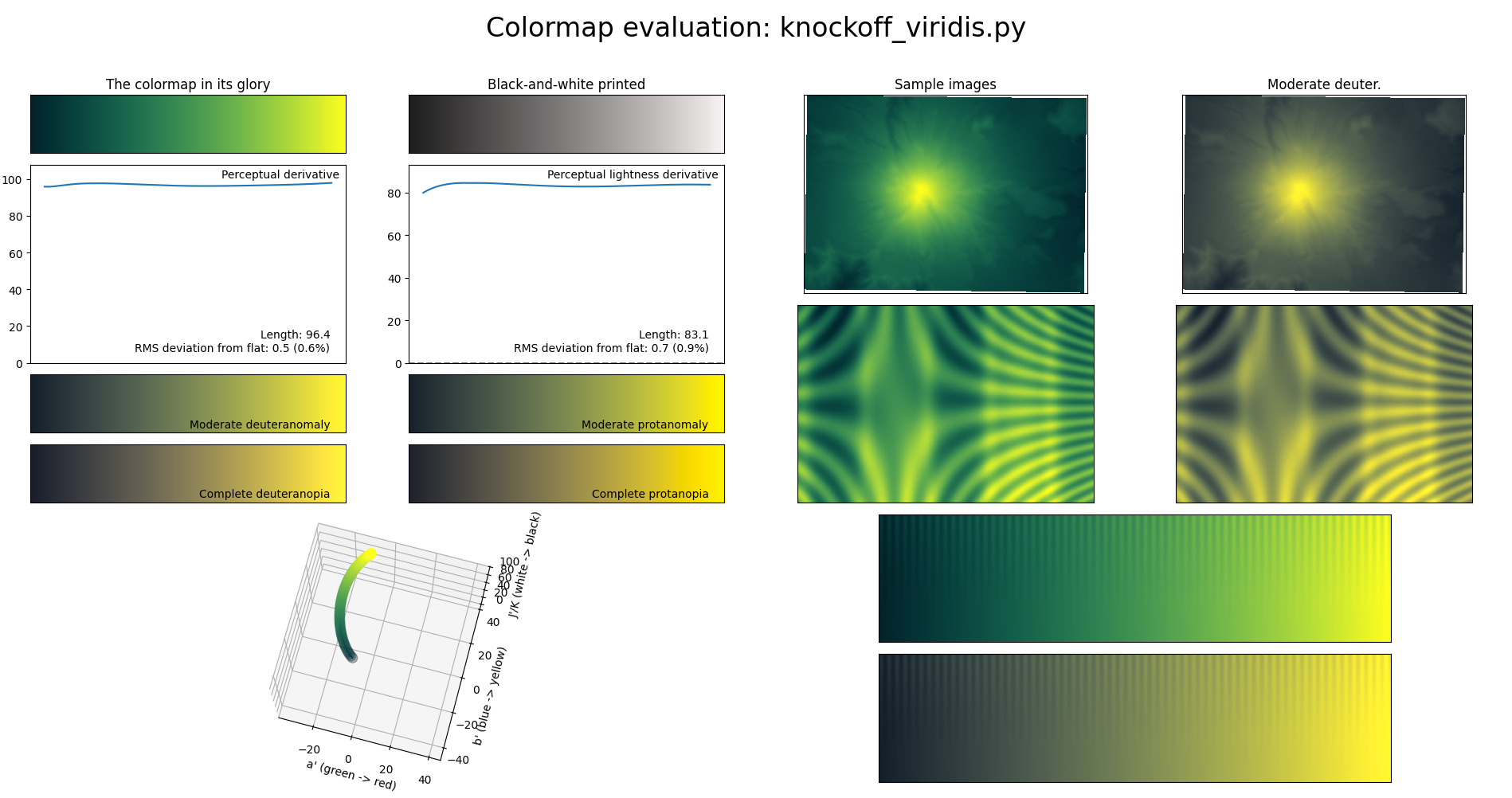
We could try something even fancier, where we optimize the coefficients of a low-degree polynomial to be close to viridis but also have low perceptual uniformity derivative, i.e. we optimize a loss function that combines distance from viridis with the same metrics used to evaluate colormaps above. This is no longer linear programming; I think I just tried random hillclimbing with a bunch of random variations on the loss function, starting from the quadratic approximation of viridis produced by the above code. Here’s my favorite result:
def knockoff_viridis(t):
    return [
        (+0.994*t - 0.009)*t + 0.014,
        (-0.031*t + 0.895)*t + 0.135,
        (-0.726*t + 0.682)*t + 0.161,
    ]
It’s pretty different from viridis and uses color much less effectively, but for being so simple, I think the curves are pretty good.
Obviously, there are all kinds of tweaks you can make to the loss function, the optimization process, and the degree of the polynomial, but I decided that I had generated enough different options to call it a day. (As with the original viridis, all the colorschemes and code in this post are dedicated to the public domain / CC0.)