I participated in the AGI Safety Fundamentals program recently. The program concludes with a flexible final project, with the default suggestion of “a piece of writing, roughly the length and scope of a typical blog post”, so naturally, I deleted all but the last two words and here we are.
When I previously considered machine learning as a field of study, I came away with an impression that most effort and computation power was going into training bigger, more powerful models; whereas the inner workings of the models themselves, not to mention questions like why certain architectures or design choices work better than others, remained inscrutable and understudied. This impression always bothered me, and it definitely influenced me away from going into AI as a career. Of course, there are important, objective safety concerns around developing and designing models we don’t understand, many of which we discussed in the program; but my discomfort is mostly a completely unrelated nagging feeling I get whenever I’m relying on things I don’t understand.
After the program and all the concurrent developments in AI (including AlphaCode, OpenAI’s math olympiad solver1, SayCan, and, of course, DALL-E 2), I still had this impression about the field at a very high level, but I also became more familiar with the subfield of interpretability — designs and tools that allow us to understand and explain decisions by ML systems, rather than treating them as black-boxed mappings from inputs to outputs — and confirmed that enough people study it to make it a thing. One quote from a post on the views of Chris Olah, noted interpretability researcher, captured my feeling particularly eloquently:
interpretability is very aligned with traditional scientific virtues—which can be quite motivating for many people—even if it isn’t very aligned with the present paradigm of machine learning.
I found the whole post insightful, and it happens that the bits before that in the passage were also relevant to me. I don’t have access to lots of compute!
Inspired by that post and by a desire to actually write some code (which I figured might help me understand the inner workings of modern ML systems in a different sense), and after abandoning a few other project ideas that were far too ambitious, I decided to go through some parts of the fast.ai tutorial and riff on it to see how much progress I could make interpreting the models, and to write up the process in a blog post. I tried to capture my experience holistically, bugs and all, to serve as a data point for what it might feel like to start ML engineering (for the rare individuals with a background and inclinations just like mine2), and maybe entertain more experienced practitioners or influence their future tutorial recommendations. A much lower-priority goal was trying to produce “my version of the tutorial”, which would draw more liberally from an undergraduate math education3 and dive more deeply into technical details.
Technical setup
The tutorial has detailed instructions on possible platforms to use, and initially, I was intimidated by how it read:
We strongly suggest using one of the recommended online platforms for running the notebooks, and to not use your own computer, unless you’re very experienced with Linux system adminstration and handling GPU drivers, CUDA, and so forth.
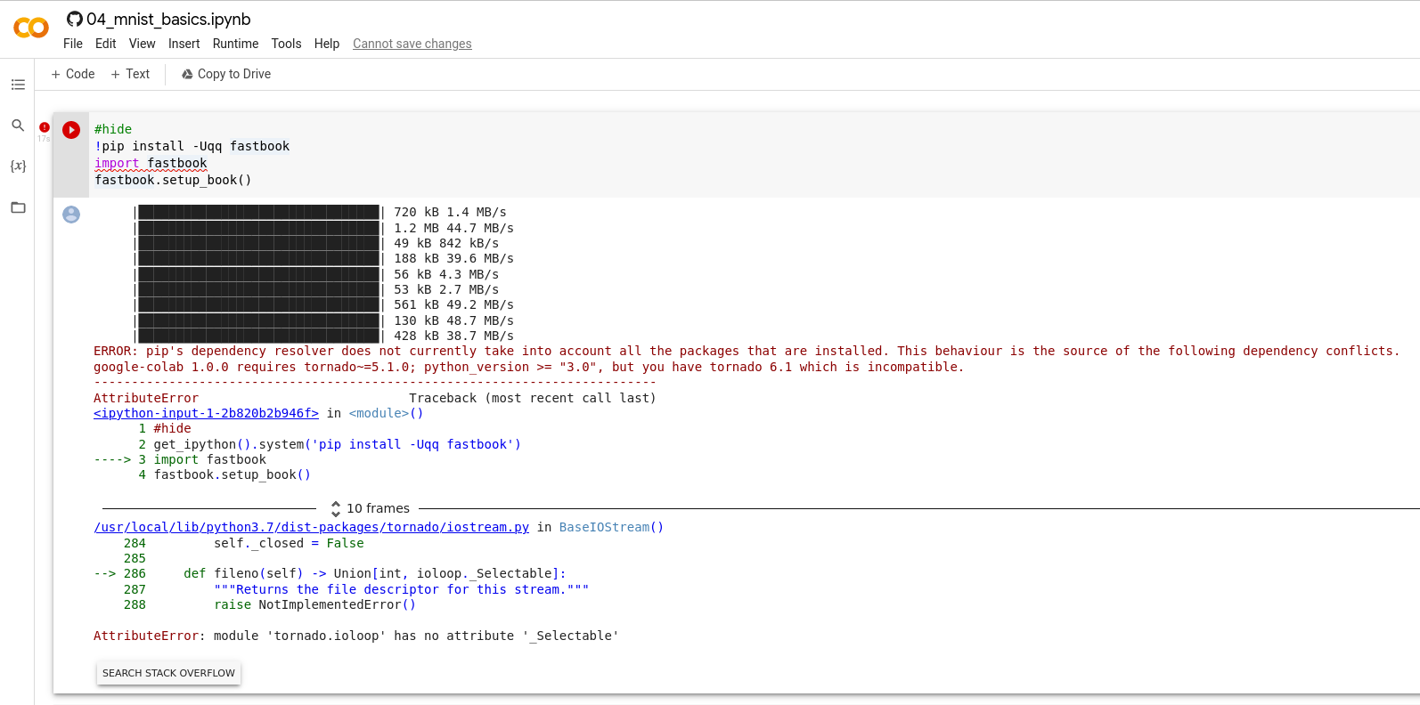
However, my personal experiences with two suggested platforms, Gradient and Colab, were both horrible. In both, the UI would regularly freeze or throw errors that I didn’t know how to debug because there was a notebook in the way, whereas I know how to debug installing Python packages on my computer.
I think there is a reasonable chance all this was caused by using the
free tier4 and not being ready to commit, but I
was not in fact ready to commit. I entertained the thought of giving up
on implementation right there and just writing something more
theoretical, but the 04_mnist_basics.ipynb notebook I was
spending the most time on opened with a little spiel about not giving
up, staring me in the face…
The story of deep learning is one of tenacity and grit by a handful of dedicated researchers.
So I decided to try just running everything on my laptop. In fact,
after looking at the secondarily recommended Anaconda installer and
being a little skeeved out by the binary embedded in the shell script, I
decided to stick with technologies I was familiar with all the way5 and just use pip.
Somewhat ironically, because my laptop doesn’t have a good GPU6 and I was not ambitious enough to want to need one, I expected that it would be easier for me to get things working, as getting code to talk to GPU drivers seemed like a big source of difficulties. And indeed, I installed all the fast.ai libraries and a Jupyter notebook without much trouble. (I even considered not using a notebook at all, and just editing a Python script and rerunning it, but it took me about five minutes of trying that before deciding that trying to implement my first few neural nets without the easy interactivity would be a disastrous impediment.)
It is my personal opinion that, if you’re not ambitious about big data, you can delete the word “very” from the tutorial’s “unless you’re very experienced with Linux” carveout. The following algorithm was basically all I needed to get PyTorch and fast.ai working:
- Try to install a package.
- If there’s an error message, paste it into your favorite search engine.
- Follow the instructions in the first StackOverflow result.
- Go to step 1.
To be fair, the algorithm probably understates the difficulty a bit.
Sometimes you have to adapt the StackOverflow answer for your
environment, or use the second answer instead if the first one is too
old. Right now, pip3 and python3 point to
different Python versions on my system, something I just haven’t felt
bothered enough to deal with, so I sometimes replace pip
with python3.10 -m pip. Because I use fish shell, I have to add
.fish to . venv/bin/activate instructions. And
so on. But I still wouldn’t call myself “very” experienced.
Anyway, with the libraries setup, it’s time to dive in.
MNIST
I decided to build a digit classifier, like in Chapter 47 (link to Colab notebook) — riveting, I know. At least, I wanted to use the full MNIST dataset instead of the toy dataset with 3s and 7s in the book. fast.ai’s External data page explains how I can acquire it, and by running this on my own computer, I can even print the actual path that this data got untarred to:
from fastai.vision.all import *
path = untar_data(URLs.MNIST)
pathPath('/home/akriloth/.fastai/data/mnist_png')Because this is on my own computer, I can actually cd to
and ls this directory, instead of trying to figure out how
to use the pathlib.Path API (as monkey-patched
by fast.ai itself — monkey-patching? In my Python library?) I
found this a lot more comfortable.
Fun fact 1: “MNIST” stands for “Modified National Institute of Standards and Technology”. None of the letters describe how the dataset has handwritten digits, or that it’s a dataset at all.
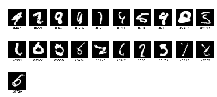
Fun fact 2: Some of the digits are horrible. Wikipedia refers to j05t’s digit recognizer on GitHub, which comes with a fascinating array of digits that it “fails to identify”:
Incidentally, while cross-referencing other tutorials, I noticed that the PyTorch tutorial uses Fashion-MNIST, which is an attempt to replace MNIST as an elementary machine learning dataset — maybe for reasons like the above? Still, I was more interested in handwritten digits since humans are great at recognizing them but not so great at describing how they recognize them, so I decided to stick with MNIST.
The untar_data step is idempotent, so it’s safe to put
in a notebook where we might run it multiple times; and we can still
look at an image in our notebook with something like:
zero_ims = (path/'training'/'0').ls()
zero_im = Image.open(zero_ims[0])
zero_im
Or we can cd to it and use whatever image viewer we
please. I usually reach for gthumb these days. Anyway,
let’s convert the images to PyTorch tensors.
training = {}
testing = {}
for digit in range(10):
    print('loading', digit)
    training[digit] = [tensor(Image.open(im_path)).float()/255 for im_path in (path/'training'/str(digit)).ls()]
    testing[digit] = [tensor(Image.open(im_path)).float()/255 for im_path in (path/'testing'/str(digit)).ls()]
A PyTorch tensor is a multi-dimensional homogeneous array of numbers, similar to a numpy array and supporting similar broadcasting semantics. Here, we divide a tensor by an integer to divide each element by that same integer. Howver, PyTorch tensors have a lot more “magic” in them than numpy arrays. Roughly, the main feature of interest is that PyTorch tensors “remember how they were computed” in order to support an automatic differentiation system, or autograd. But more on that later; for the time being we can treat them as oddly named numpy arrays.
The images have pixels from 0 to 255. We’re going to convert them to floats in \([0,1]\) right away, so we don’t forget to do so later. I did, in fact, forget to do so while iterating on the code in this post, and ended up with some great bugs.
Absolute difference from mean
The first toy model we make in the fast.ai course is as follows: For each digit, take the average of every training image showing that digit to get an “ideal digit”. To predict what digit a future image is, we’ll just compute its distance to each “ideal digit” and pick the closest one. For the distance we’ll also follow the course and use the sum of absolute values of elementwise differences, i.e. the L¹ norm. However, the tutorial only does it for 3 and 7. Let’s do the analogous thing for all ten digits in our full data set.
I don’t think I would describe this as machine learning, exactly. It’s just “machine”. Still, I found it useful practice.
Average zero:
z = torch.stack(training[0]).float()torch.stack has type
Sequence[tensor] -> tensor. I didn’t know that Python
actually sort-of-formally defines “sequence”
— it’s an iterable that supports integer indexing and len.
Then, we call mean, which takes an axis argument.
show_image(z.mean(0))Unlike the mundane digits in the course, my 0 had a vaguely psychedelic color scheme.

It turns out this was because I hadn’t run the configuration step
matplotlib.rc('image', cmap='Greys') beforehand. The scheme
depends on the colormap
chosen by matplotlib; the default is called viridis and
has a lot of careful
thought behind it. (2024
update: I wrote a whole other
post about it.) Honestly, I kinda like it.
Now that we know this works, let’s make all of the average digits.
training_means = torch.stack([
    (torch.stack(training[digit]).float()/255).mean(0)
    for digit in range(10)
])
This is a 10 × 28 × 28 tensor. If we had a
28 × 28 tensor im, how do we neatly compare it
against each of these means and figure out which mean has the smallest
sum of absolute differences from im?
(im - training_means).abs().mean((1, 2)).argmin().item()When we compute im - training_means, the former is
28 × 28 and the latter is 10 × 28 × 28, so the
former broadcasts and we get a 10 × 28 × 28 tensor of
differences. Then, we take its elementwise absolute value, and then we
compute the mean along axes 1 and 2 (0-indexed), i.e. the two length-28
axes. The result is a length-10 tensor. Finally, we take
its argmin, the index at which the value is minimal.
Finally finally, we have a zero-dimensional tensor with a number in it,
but we want to get the underlying Python number out because it prints
more nicely; .item() accomplishes this. (This is another
difference from numpy, where argmin and similar operations
would directly return scalars,
but it makes sense in PyTorch’s case because scalars need to “remember
how they were computed” just as much as higher-dimensional arrays.)
To see how this model performs, let’s define a function for analyzing the accuracy of any predictor, so we can reuse it later:
def show_results(predictor):
    for name, data in [('testing', testing), ('training', training)]:
        print('results on', name)
        total_correct = 0
        total_total = 0
        for i in range(10):
            correct = 0
            total = 0
            for im in data[i]:
                correct += predictor(im) == i
                total += 1
            print(i, ":", correct, '/', total, '=', correct/total)
            total_correct += correct
            total_total += total
        print(total_correct, '/', total_total, '=', total_correct/total_total)
If we assume the predictor works elementwise, we could
optimize this function a lot, but I deliberately avoided it to try to
minimize the risk of bugs in this function. We don’t run it often
anyway.
Much later, I realized that show_results is already the
name of a function that fast.ai imports into the global scope, but I
decided not to change my function’s name to faithfully represent my
experience.8 To be honest, I don’t even
understand why show_results is in scope; all the
documentation I could find only have it as a method on various classes.
Something type
dispatch something? Anyway, we can use it like so:
show_results(lambda im: (im - training_means).abs().mean((1, 2)).argmin().item())My closest-average code gets 66.85% accuracy on the test set and 65.13% on the training set. In theory, this is completely deterministic.
Remember the bug I mentioned? When I first wrote this code, my prediction did something equivalent to:
show_results(lambda im: (im - training_means/255).abs().mean((1, 2)).argmin().item())This actually got higher accuracies of 72.44% and 71.18%. If avoiding and noticing these bugs is what machine learning engineering proficiency is about, it’s obviously something I don’t have (yet).
Creating a trivial linear model
We’re going to make the simplest neural network possible: a single layer of 10 neurons, each with weights and a bias and corresponding to a possible digit. I’m not sure if this even counts as a neural network, actually, but I guess we will add a nonlinearity at the end to interpret the outputs as probabilities.
Let’s start by getting all our data into PyTorch tensors.
train_x = torch.cat([t.float()/255 for i in range(10) for t in training[i]]).view(-1, 28*28)
train_y = tensor([i for i in range(10) for _ in training[i]])
train_x.shape, train_y.shape
First, we concatenate
all the training images. Next, we view
the resulting tensor as a two-dimensional vector whose second dimension
is 28 × 28 = 784, and first dimension is unspecified; -1
means “pick whatever number makes the size work out”. This flattens each
training image, originally a 28 × 28 tensor, into one length-784 vector,
and gives us a tensor whose rows are those vectors.
view always gives a tensor that’s backed by the same
memory as the tensor you call it on, so mutating either tensor affects
the other. However, view might fail if this isn’t possible.
The documentation is a little inscrutable, but most tensors can be
viewed as any shape with the same size (number of
elements). Tensors that can’t are non-contiguous
(this answer is about numpy but the same principles apply) and will most
often arise by transposing existing tensors, though being non-contiguous
only prevents view-ing the non-contiguous dimensions.
I also deviated a little from the fast.ai tutorial, which calls
.unsqueeze(1) on train_y. unsqueeze
is one of the rare PyTorch functions whose name differs from its numpy
counterpart, expand_dims;
it adds an axis, specified by the new axis’s (0-indexed, as usual)
dimension. Here, it would convert the one-dimensional length-n
tensor into an n × 1 tensor. I haven’t figured out the rationale
for doing this, and not doing it seems to make our lives a
little easier later.
Actually, this kind of thing essentially caused the one bug I remember writing in that one machine learning course. Somewhere deep in my code, I did something like elemmentwise-multiplying a 10 × 1 array by a one-dimensional length-10 array, which broadcast them to produce a 10 × 10 array, and then computing the sum of the result. Naturally, that sum was wildly off with the value I actually wanted, which was the sum of the 10 elements of the elementwise product of the two arrays, and I didn’t notice it for the longest time.
Now we’re going to define our one layer, an affine transformation \(\mathbb{R}^{784} \to \mathbb{R}^{10}\), as a matrix of weights (to multiply the input by) and a vector of biases (to add at the end).
def init_params(size, std=1.0):
    return (torch.randn(size)*std).requires_grad_()
weights = init_params((28*28, 10))
bias = init_params((10))
I glossed over the exact code in the tutorial here and got very tripped up later when my tensor sizes didn’t match up. If you’re familiar with linear algebra, you may be used to thinking of any given \(n \times m\) matrix \(M\) as a linear transformation \(\mathbb{R}^m \to \mathbb{R}^n\), given by \(x \mapsto Mx\). Matrix multiplication \(A \mapsto MA\) can then be interpreted as applying the linear transformation \(x \mapsto Mx\) column-wise to \(A\). That’s how I think of it, at least.
The problem is that this requires us to consider \(A\) as a sequence of column vectors, and
PyTorch tensors (and numpy arrays, and so on) don’t really “want to” be
thought of this way. A two-dimensional tensor “wants to” be considered
as a sequence of row vectors, since you get row vectors when you iterate
over it and when you index into it once; in fact, this works better with
other aspects of mathematical notation, since matrix dimensions usually
list the number of rows first and \(M_{ij}\) usually means the \(i\)th row, \(j\)th column, matching
m[i][j].
It’s possible to cling to our column-oriented mathematical intuition
by sprinkling transposes everywhere in our code, but after thinking this
through more I decided that, overall, it’s easier to get used to \(n \times m\) matrices as actually
representing transformations \(\mathbb{R}^n
\to \mathbb{R}^m\) via \(x \mapsto
xM\), and to apply such matrices by multiplying them on the
right. Hence why my weights has dimensions \(784 \times 10\) instead. To the
mathematician, this is all obviously isomorphic anyway.
With the long aside on matrix shapes out of the way, the other stuff going on in this code is that:
randngenerates a tensor of the specified size, and fills it with random numbers from a normal distribution with mean 0 and variance 1requires_grad_()marks that we will want to compute the gradient with respect to this value. The trailing underscore is a PyTorch convention that the method mutates the tensor in-place rather than returning a copy or view. This function is the first step to using the PyTorch autograd system I alluded to when introducing tensors.
Before we do that, though, let’s try predicting with our uninitialized, completely random model:
show_results(lambda im: (bias + im.view(28*28) @ weights).argmax().item())The result of this will actually be quite random, but I did get
around 10% accuracy on both datasets. You may notice widely varying
accuracies on digits, which I was briefly surprised by but quickly
understood to be caused by the random bias — the random
model is predisposed to predict certain digits much more often than
others, so it will naturally get those digits right more often.
Training the trivial linear model
For completeness, I’ll recap the techniques and choices made by the
fast.ai tutorial I’m copying (and which I understand to be very standard
in ML): We want to optimize our model with gradient descent,
where we take some function of our model we want to optimize, compute
its derivative with respect to each parameter in our model (that is,
each weight and bias), adjust each parameter in the direction suggested
by that derivative, and repeat. To do this, we need a differentiable
function to optimize. Accuracy isn’t differentiable (or rather, its
derivative is 0 almost everywhere because it’s discrete-valued and a
“step function” at its core), so instead we consider the softmax of the
vector output by our model. Abstractly, softmax is the \(\mathbb{R}^n \to \mathbb{R}^n\) function
\[\text{softmax}(z_1, \ldots, z_n) =
\left(\frac{e^{z_1}}{e^{z_1} + \cdots + e^{z_n}}, \ldots,
\frac{e^{z_n}}{e^{z_1} + \cdots + e^{z_n}}\right).\] The \(i\)th component can be thought of as a
continuous version of “whether the argmax equals \(i\)” (hence the name “softmax”): \[\frac{e^{z_i}}{e^{z_1} + \cdots + e^{z_n}}
\approx \begin{cases} 1 & \text{if }z_i = \max(z_1, \ldots, z_n) \\
0 & \text{else} \end{cases}.\] Note also that softmax’s
outputs are always in \([0, 1]\) and
that the sum of the components of a softmax is always 1, which are other
ways it’s like argmax (assuming ties are broken deterministically) and
which we’ll come back to later. By replacing the “argmax equals \(i\)” condition in our
show_results function with this function, we can go from
computing the discrete-valued accuracy to computing a continuous-valued
“accuracy, but it’s continuous”.
PyTorch comes with a softmax function, so we can take
the softmax of our model’s outputs on the very first training image
with:
torch.softmax(bias + train_x[0] @ weights, dim=0)The result is a length-10 vector. Because train_x is in
order, the correct digit for this image is 0, so the first
(that is, 0th) element of this vector represents “whether our model got
the answer right, but it’s continuous”.
To apply our model to every single image at once, we can just write
bias + train_x @ weights. If we had a GPU, this is the kind
of thing it would parallelize very effectively. Then we can
softmax across each row, index out all the elements
corresponding to the correct answers, and compute their average. I
couldn’t find exactly where PyTorch documents this, but (I assume) it
works just like what numpy calls advanced
indexing.
torch.softmax(bias + train_x @ weights, dim=1)[range(60000), train_y].mean()The event that prompted me to think really hard about tensor shapes
was that I tried writing the above when train_y had been
unsqueezed and was a 60000 × 1 tensor. My notebook promptly
crashed. I believe this was because advanced indexing broadcasts the
tensors being indexed with, resulting in trying to index into the tensor
of softmaxes with 60000 × 60000 pairs. Unwanted
broadcasting strikes again!
Anyway, this “continuous accuracy” is also close to 0.1.
However, this value still won’t be the function we try to optimize
directly. Why not?
A glib response is that, if you try optimizing it, it “doesn’t work”; the accuracy doesn’t really go up. A longer explanation is that making our accuracy differentiable doesn’t mean that we’ve made it suitable for gradient descent. Just as accuracy’s derivative is 0 almost everywhere, softmax’s derivative is approximately 0 approximately almost everywhere, so the gradient will often fail to provide a strong signal on which way to adjust the parameters.
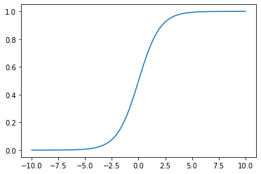
x = np.linspace(-10, 10, 100); plt.plot(x,
1/(1+np.exp(-x)))
)
When we evaluate the model, it makes sense to award 0 points for being wrong and 1 point for being right because the result represents accuracy, a concept we’re familiar with; but when we train the model, we want gradient descent to change parameters when the model is wrong and not change them when the model is right, so we sort of want to artificially punish being wrong more than we want to reward being right.
I think this is a fairly satisfying answer for why we don’t optimize the softmax directly, but to explain the choice of function we do optimize requires a longer diversion.
What is entropy?
For a random variable \(X\) with outcomes \(x_1, \ldots, x_n\), the entropy of \(X\) is given by \[H(X) = -\sum_{i=1}^n P(x_i) \log P(x_i).\] Entropy is a nonnegative quantity because probabilities are between 0 and 1, so their logs are negative. That’s fine and all, but I’m not here to regurgitate definitions, I’m here to try to explain them and convince you (and myself) that they make sense.
There are many interpretations of entropy, but the one that eventually made sense to me in this context is that entropy is a way to quantify the expected amount of “surprise”. When you experience an event with probability \(p\), we might say that you experience \(-\log p\) units of surprise. This formulation already runs counter to typical usage since it implies that there’s no way to not be surprised when experiencing a random event. For example, if you just flip a coin over and over and keep observing the result, by our definition, you’re constantly experiencing \(\log 2\) units of “surprise” per flip; whereas any normal human flipping coins over and over would probably be bored out of their mind. But let’s ignore that aspect.
It makes sense that less likely events are more surprising, but why do we use the log instead of any other decreasing function, say \(1/p\)? A short response is that it makes sense for winning the lottery twice to be twice as surprising as winning it once. Or does it? I have thought about this for long enough that I no longer know if this appeal to common sense holds any water.
A slightly longer response, which also links entropy back to our machine learning context, is as follows: We are trying to build a system that can predict events. If you’re trying to predict events, you could informally describe your predictor as being “surprised” when it makes a prediction and the prediction turns out to be wrong; “surprise” is therefore bad, and is a quantity you want to minimize. Now, suppose you have some candidate systems for predicting two independent random variables, and you want to construct a system to predict both random variables at the same time. Then it would make sense for the best candidate for that task to just be a combination of the best candidate for predicting each individual random variable. By adopting entropy as your definition of surprise, any candidate’s “expected surprise” will just be the sum of its “expected surprise” on the first and second variables, so it’s optimal to combine the best candidates for predicting the individual variables, as desired.9
Now that we understand entropy, we can understand some useful related terms. The cross-entropy between two probability distributions \(P\) and \(Q\), or more precisely the cross-entropy of \(Q\) relative to \(P\), is the expected value of surprise you experience if you believe the probability distribution is \(Q\) when it’s actually \(P\): \[H(P, Q) = -\sum_{i=1}^n P(x_i) \log Q(x_i).\] That is, we say you experience “surprise” based on how probable you think the outcome is, but calculate expected value based on how probable the outcome actually is.
The Kullback–Leibler divergence is the “excess” expected amount of surprise you experience if you believe the probability distribution is \(Q\) when it’s actually \(P\): \[\begin{align*}D_{\text{KL}}(P, Q) &= H(P, Q) - H(P) \\ &= -\sum_{i=1}^n P(x_i) (\log Q(x_i) - \log P(x_i)).\end{align*}\] When I say “excess”, I’m implicitly relying on an assumption that, for fixed \(P\), the cross-entropy \(H(P, Q)\) is minimal when \(Q = P\); that is, when you believe that the probability distribution is what it actually is, you’re minimizing the expected value of surprise you’ll experience when you observe the random variable. This fact is not obvious! For a different definition of entropy or surprise, you could totally imagine the math working out so that, say, somebody who believes unlikely events are even more unlikely than they actually are comes out ahead in terms of minimizing surprise. But the fact that this doesn’t happen for our definitions is known as Gibbs’ inequality.
This is good for our use cases in that, if we have a system that produces a probability distribution \(P\), minimizing either cross-entropy or the Kullback-Liebler divergence of \(P\) relative to some actual probability distribution \(Q\) can be considered as trying to get the system to have “true beliefs” about the probability distribution.
Is this the correct way to think about entropy?
This is a massive tangent that you should probably skip.
Haskell has a fun concept called monads:
class Monad m where
    (>>=)  :: m a -> (a -> m b) -> m b
    return :: a -> m a
I will not explain them here because that’s not the point, but they
are widely considered to be an infamously difficult concept to
understand in Haskell, and hundreds of tutorials have been written about
them trying to give intuitive explanations what they “really are”.
Unfortunately, there really isn’t anything in most other programming
languages, computational models, or the experiences of most Haskell
newbies that are a perfect analogy for monads. If monads are containers,
why can’t you get the value contained by an IO? If monads
capture side effects, what is the free monad and how does Tardis actually
send side effects backwards in time? The idea that, after you’ve gotten
an intuitive grasp for a new concept, you can explain your intuition in
a tutorial and the reader will immediately understand it just as well,
has been dubbed the “monad
tutorial fallacy” in this context.
In the end I think the only really correct way to think of “monad” is
“something that supports
>>= :: m a -> (a -> m b) -> m b and
return :: a -> m a10”, and the only way to
understand “monad” is to think about that assertion and about various
examples until it makes sense.
This is my long-winded way of saying that, although I feel like I “understand” entropy a lot better after writing the previous section, it might not really be a shortcut for anybody else staring at \[H(X) = -\sum_{i=1}^n P(x_i) \log P(x_i)\] and playing with it until it makes sense.
On the other hand, this section may also just be an overreaction to a pedagogical phenomenon that’s way rarer than I think it is, a la “Guy who has only seen The Boss Baby”. So who knows.
Actually choosing our loss function
Where we left off, we had computed all the correct elements of softmaxes:
torch.softmax(bias + train_x @ weights, dim=1)[range(60000), train_y]We also explained why optimizing their mean isn’t what we want. Instead, we will be optimizing for their negative log:
-torch.log(torch.softmax(bias + train_x @ weights, dim=1)[range(60000), train_y]).mean()To make fully explicit the connection here to our long sidebar on entropy, we observe that softmax outputs a vector of positive reals that sum to 1, so we can interpret that vector as a probability distribution — how likely the model believes the image is to be each of the digits. In that case, the negative log of the softmax component corresponding to the correct answer is “how surprised” the model would be when we reveal the true digit corresponding to the image is. This can also be thought of as the cross-entropy of the model’s probability distribution relative to the true distribution of the digit, the latter of which is just that that digit is what it’s labeled as 100% of the time. A perfect model would always assign 100% probability to the correct digit and experience 0 surprise; but note that if that model were to be 100% confidently wrong about even one single digit, it would be infinitely surprised.
In this ML context, the function we optimize for is called a “loss
function”, and fast.ai’s nn has a loss function for this, so
we could have just written:
nn.CrossEntropyLoss()(bias + train_x @ weights, train_y)You can also pass reduction='none' to recover the tensor
of negative logs of individual softmax components:
nn.CrossEntropyLoss(reduction='none')(bias + train_x @ weights, train_y)With the loss function locked down, we only need one more thing to train our model, the optimization process itself.
Stochastic Gradient Descent
We could perform gradient descent by directly taking the expression for cross-entropy loss we got above, telling PyTorch to compute all the gradients, adjusting our parameters, and repeating.
However, this makes every step very slow, since PyTorch will have to look at how every single training image and label affects the gradients; and we want to perform many steps of gradient descent, because the function we’re optimizing is nonlinear and the gradient should change a lot after each step. (If it were linear, there would be no need for gradient descent at all. We could just consider each parameter individually and set it to the extremum that optimizes our objective function.)
Instead, we compute each gradient descent step using a random subset of our training data – hence, stochastic gradient descent. We’ll just copy the tutorial and use PyTorch’s DataLoader, since code to choose many random subsets of a set isn’t particularly interesting.
The same documentation lists some dataset classes that we could have used, so we could have avoided loading all the MNIST images into Python and converting them to tensors; but I guess it was educational. We also can get by very easily without the PyTorch dataset classes at all, because a dataset is just a sequence of (x, y) pairs:
A custom Dataset class must implement three functions:
__init__,__len__, and__getitem__.
So we can make a dataset and a data loader like this:
dset = list(zip(train_x, train_y))
dl = DataLoader(dset, batch_size=256, shuffle=True)
Each time we iterate over the DataLoader, it will
shuffle the data, divide it into size-256 batches, and serve them to us
one by one. As a demonstration, we could get one batch with first.
Because of course fast.ai comes with such a helper.11
batch_x, batch_y = first(dl)Now we can finally perform one step of gradient descent. First, we
compute the gradients with the magic function tensor.backward:
nn.CrossEntropyLoss()(bias + batch_x @ weights, batch_y).backward()Remember, when I first described PyTorch tensors, how they “remember
how they were computed”? It’s all for this call. Calling
backward computes the gradient of the quantity you call it
on with respect to each graph
leaf — basically, the tensors we created and called
.requires_grad_() on. It records those gradients by
mutating the .grad
property of each graph leaf, initializing that attribute to the zero
tensor if necessary and then adding the computed
gradient to that tensor. (It then deletes the relevant
computation graph, that is, the information about how tensors were
computed; we could have kept it by passing
retain_graph=True.)
Note that this means that we’re responsible for zeroing or deleting
grad from each of our parameters between steps! Why does
backward work this way? This PyTorch
forum discussion goes into some example use cases where you want to
accumulate gradients over multiple backward calls, but why
is it the default behavior instead of something you enable by passing a
flag to backward? I don’t have a satisfactory answer, but I
also haven’t really gone through that entire discussion in detail. It
does seem like a popular footgun though.
In any case, after backward deposits the computed
gradients on the tensors representing our parameters, we can adjust the
parameters with them. We subtract the gradients because we are trying to
minimize our loss function, plus we have to pick a learning
rate — a constant to multiply the gradient by to decide how much to
change each parameter by — but we’ll deal with that later and pick the
trivial 1. Then, we clean up after ourselves to avoid the footgun.
bias.data -= bias.grad # * lr
weights.data -= weights.grad # * lr
bias.grad.zero_()
weights.grad.zero_()
And that’s one step! All together now, here’s how we can optimize our model for ten epochs with a learning rate of 10. In the machine learning training process, an epoch refers to one pass through the full training data set, in whatever order or batches we choose.
lr = 10
for i in range(10):
    for batch in dl:
        batch_x, batch_y = batch
        nn.CrossEntropyLoss()(bias + batch_x @ weights, batch_y).backward()
        bias.data -= bias.grad * lr
        weights.data -= weights.grad * lr
        bias.grad.zero_()
        weights.grad.zero_()
    print(nn.CrossEntropyLoss()(bias + train_x @ weights, train_y))

show_results(lambda im: (bias + im.view(28*28, 1) @ weights).argmax().item())
In practice, ten iterations is not nearly enough to get a good model. Instead of trying to pick the learning rate with a more principled approach, such as the “learning rate finder” described halfway through Chapter 5, I decided to just try some random numbers… and then accidentally spent an hour or so just repeatedly running this cell in my notebook, tweaking the learning rate and number of steps and watching the loss slowly creep down. Making numbers change monotonically is my siren song.
One odd thing I experienced was that sometimes, when a low learning rate seemed to have stopped improving the loss, running a few epochs at a much higher learning rate and then reverting to the low rate would make the loss temporarily much higher but fairly reliably bring it back down to lower than the loss at which it was stuck at. I didn’t think about this very hard, but it doesn’t seem too unreasonable for local and global optima to just be that way, so I didn’t investigate in more detail. I ended up with a loss of 0.3325, a training accuracy of 90.82%, and a testing accuracy of 90.33%.
I decided to save my work. PyTorch has built-in serialization and
deserialization functions for this, called save and
load.
import datetime
now = datetime.datetime.now().strftime('%Y-%m-%d-%H-%M-%S')
torch.save(bias, f"bias-{now}.pt")
torch.save(weights, f"weights-{now}.pt")
Fun fact 3: After I did this and finished writing a lot of this post,
I went over my code again and discovered that there was still
an extra /255 lurking in my code. Consequently, when I
loaded my tensor back in and tried to connect it to my most recent code
to fetch the dataset, the accuracy was abysmal. Fortunately, I divided
my saved weights by 255 and everything was isomorphic.
Also, as a security engineer (and as somebody fresh off a CTF
challenge on this subject), I am obligated to mention that
torch.save/torch.load use Python’s pickle
internally, and it is trivial to construct data that executes
arbitrary code when unpickled. (PyTorch may error with
Invalid magic number; corrupt file? afterwards, but by then
it’s too late.)
import io, os, pickle
class Exploit:
    def __reduce__(self): return os.system, ("echo 'get hacked lol'",)

torch.load(io.BytesIO(pickle.dumps(Exploit())))
I don’t recommend calling torch.load on files from
untrusted sources.
Interpreting our model
Let’s try to understand what’s going in our simple neural network.
fast.ai has some really nice utilities for this.
show_images takes an iterable of 2D tensors. With almost no
effort, we can directly visualize the weights our training process
produced.
show_images(weights.T.view((10,28,28)))
weights
You can sort of see the digits in most of these neurons.
Since this is so easy, we can investigate what happened earlier when we tried optimizing softmax directly. The results are really interesting! Here’s an example run:

weights from an attempt to train our model’s
softmax-based accuracy directly
The training process seems to have randomly “burned in” a few digits from the training set in each weight matrix. Although I didn’t investigate this in as much detail as I’d have liked to, I think my earlier hypothesis was roughly correct: doing gradient descent the softmax directly only makes significant steps when the model happens to be close to 50% confident about the correct digit, because that’s where the gradient is nonzero. This happens rarely and unpredictably, so the neural network reacts strongly to individual images that “got lucky”, resulting in these weights.
Back to our “good” model now. I cribbed off Feature Visualization for other ideas on what to do. One idea is simply to look for the images in the dataset that the model most confidently recognizes as each digit:
examples = []
labels = []
for digit in range(10):
    confidences = torch.softmax(bias + train_x @ weights, dim=1)[:,digit]
    conf = confidences.max().item()
    bi = confidences.argmax().item()
    examples.append(train_x[bi].view((28,28)))
    labels.append(f"{digit} ({conf*100:.02f}%)")
show_images(examples, titles=labels)
I switched back to the Greys color scheme to show these
tensors since we’re actually analyzing them as inputs to our model.
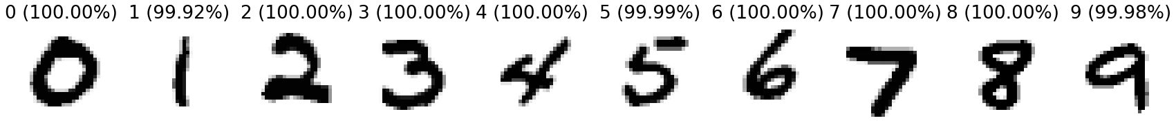
I think these images make a lot of sense: bold, clear strokes to provide a strong signal.
Something creative we could do is to visualize the gradient of the
loss with respect to each pixel in the image, superimposed on the images
themselves. One small detail here, which isn’t strictly necessary but I
think is good to know about, is that we call detach on our
tensors to get detached copies that aren’t connected to the graph of
computations and don’t have requires_grad. Without this,
each time we calculate the gradients with backward to
compute a gradient, it will also calculate the gradients for
bias and weights, which is both wasteful and
can cause errors if bias/weights are not
directly graph leaves, because backward also deletes the
computation graph. I also slam some
clone/detach/requires_grad_ on
the image tensor itself just to be safe; all our tensors are small so it
doesn’t matter.
bias = torch.load('bias-2022-05-02-00-42-40.pt').detach()
weights = torch.load('weights-2022-05-02-00-42-40.pt').detach()
examples = []
for digit in range(10):
    confidences = torch.softmax(bias + train_x @ weights, dim=1)[:,digit]
    print(confidences.shape, confidences.min(), confidences.max())
    conf = confidences.max().item()
    bi = confidences.argmax().item()
    img = train_x[bi].clone().detach().requires_grad_()
    torch.softmax(bias + img @ weights, dim=0)[digit].backward()
    x = 1 - img.view((28,28))
    g = img.grad.view((28,28))
    g /= g.abs().max()
    # g = -1 -> (0,0,0.5) (0.5,0.5,1)
    # g =  0 -> (0, 0, 0) (1,  1,  1)
    # g = 1  -> (0.5,0,0) (1,0.5,0.5)
    base = torch.stack([-g.minimum(tensor(0))/2, torch.full((28,28),0), g.maximum(tensor(0))/2])
    delta = 1 - g.abs() / 2
    examples.append(base + (1 - img.view((28,28))) * delta)

show_images(examples)
I believe what I need to convert each (pixel, gradient) pair to a
color is a “bivariate colormap”, but I couldn’t find one in a hurry, so
I handrolled something hasty. The mapping is about as perceptually
nonuniform as it gets, but it’s enough to give us a little more insight
into the model’s behavior. Because blue means the gradient of the loss
is negative, it means a higher number in the source image (darker, in
our Greys visualization) there would the model more
confident in that digit, and red means the opposite. As a sanity check
to make sure we didn’t flip our signs, we can see that, for example,
filling in the center of the 0 or adding a stroke to most areas near the
1 would make the model less confident in those images, which makes
sense.
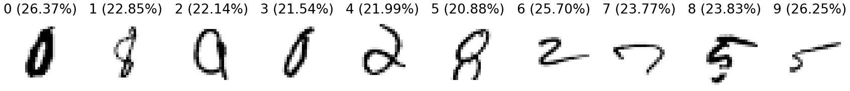
Just for kicks, we can also look at the images the model is least confident in.
We can also just optimize an image such that our model is maximally confident in its classification, using — you guessed it — gradient descent.
We can use a pretty similar setup, except we don’t need to worry
about batches and such, and we call detach a few times to
be safe. We also want to clamp the image’s components to the \([0,1]\) range to match our data without
affecting any gradients or the computation graph, so we directly
manipulate .data on our tensor.
I have no idea if this is the “correct” way to do these things in PyTorch, but, as far as I can tell, it worked.
bias = torch.load('bias-2022-05-02-00-42-40.pt').detach()
weights = torch.load('weights-2022-05-02-00-42-40.pt').detach()
# or, to get noninterfering copies of bias and weights from the same session:
# bias.clone().detach(), weights.clone().detach()
examples = []
for digit in range(10):
    example = torch.full((28*28,), 0.5).requires_grad_()
    lr = 1
    conf = 0
    its = 0
    while conf < 0.9999:
        c = torch.softmax(bias + example @ weights, dim=0)[digit]
        conf = c.item()
        torch.log(c).backward()
        example.data += example.grad * lr
        example.grad.zero_()
        example.data = torch.maximum(torch.minimum(example.data, torch.tensor(1)), torch.tensor(0))
        its += 1
    examples.append(example.view((28,28)))
show_images(examples)
lr = 1
Interestingly, the example for 1 took more gradient descent steps to reach my target confidence than the rest of the digits combined.
Unsurprisingly, these look mostly like the weights themselves. While they’re definitely pretty bizarre, you can sort of see the digits in them if you squint.
We can repeat the experiment with different learning rates:


lr = 10 and 100
respectively
These are not as great, but you can still sort of imagine the digit in many of the images.
We can also start gradient descent from a different image.

lr = 1 starting from a training 0
Since we have all this infrastructure, why not try to generate some adversarial examples?
I’ve always felt like there is or should be a deep duality between the existence of adversarial examples and AI safety. Adversarial examples are typically inputs obtained by slightly perturbing an existing input so that a model misclassifies (or mislabels, or otherwise errs) on them; but more deeply, adversarial examples are just about ways in which a neural network’s understanding diverges from human cognition or perception, because what “slightly perturbing” means is ultimately defined by the latter. If you take a 0 and change it until it looks like a 3 to the neural network, but it also now looks like a 3 to you, that’s not an adversarial example. And if we have a general way to get a neural network to not diverge from human cognition/perception, I think we’d have mostly solved AI safety.
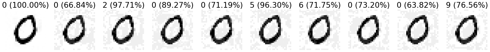
What I’m going to do is start from the first training image and then run gradient descent to optimize the classifier’s confidence that that image is some digit, as before, but also clamping each pixel to be within a fixed “tolerance” from what it was in the original image.
examples = []
labels = []
for digit in range(10):
    orig = training[0][0].clone().detach().flatten()
    example = orig.clone().detach().requires_grad_()
    upper_bound = torch.minimum(torch.tensor(1), orig + 0.25)
    lower_bound = torch.maximum(torch.tensor(0), orig - 0.25)
    lr = 1
    conf = 0
    it = 0
    while it < 10000:
        c = torch.softmax(bias + example @ weights, dim=0)[digit]
        conf = c.item()
        torch.log(c).backward()
        example.data += example.grad * lr
        example.grad.zero_()
        example.data = torch.maximum(torch.minimum(example.data, upper_bound), lower_bound)
        it += 1
    examples.append(example.view((28,28)))

    c = torch.softmax(bias + example @ weights, dim=0)
    prediction = c.argmax().item()
    confidence = c.max().item()
    labels.append(f"{prediction} ({confidence*100:.02f}%)")
show_images(examples, titles=labels)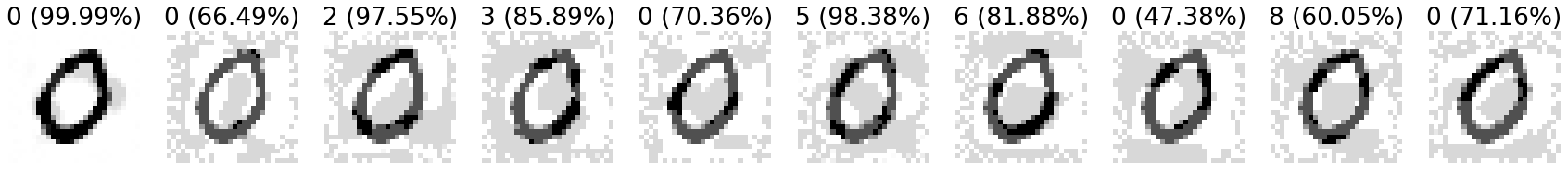
As you can see, within the tolerance I chose, I wasn’t able to get the 0 misclassified as every other digit. I tried a few tolerance levels to pick one that was around the most interesting, where the adversary succeeds for some digits and fails for others. These adversarial examples aren’t that convincing — you can definitely perceive that there’s something shady going on with them — but I think all of them still look far more like a 0 than any other digit.
The lowest tolerance for which I optimized the 0 image into being classified as something else was around ±0.15, with this image:

I must admit that I was a little disturbed to find that even our trivial neural network is clearly classifying images in ways that are bizarre to us. But while looking around on the subject, I discovered that Explaining and Harnessing Adversarial Examples, one of the earliest papers on them, already observed and more or less explained this phenomenon.
Speedrunning a “real” two-layer neural network
I feel like I could spend weeks just continuing to investigate these simple neural networks and slowly making them more complicated12; but out of a desire to have something publishable by the “preferred submission date” deadline (which has been incredibly motivating and which I expect to be much less motivating if I don’t finish by then), I’m going to speedrun through the code necessary to add a second layer and cursorily apply some of the same interpretation techniques. Consider this sequel bait.
We could, of course, just define two weights and bias tensors each,
and copy-paste all our old code to work with all four at the same time;
but I think it’s easier and more educational to just avail ourselves of
some of the abstractions PyTorch and fast.ai provide. PyTorch defines
the abstraction of modules
(not to be confused with Python modules — great job naming your
abstractions, folks), which contain parameters, specify an
input-to-output transformation, and can be trained; and it also provides
dozens of built-in modules in the nn
module-in-the-sense-of-Python. We can just specify our layers in
order as Modules: two Linear modules, which
both hold a weight and bias tensor,
sandwiching a nonlinearity, ReLU (the rectified linear
unit \(\text{ReLU(x)} := \max(0,
x)\), which definitely wins the “most jargon-y name for a simple
concept” award). Then we pass all of them to the Sequential
module.
Since I wanted to look at what each neuron was doing, I decided to use a quite small second layer, with only 20 neurons.
simple_net = nn.Sequential(
    nn.Linear(28*28,20),
    nn.ReLU(),
    nn.Linear(20,10),
)
One layer of abstraction up, fast.ai defines the Learner abstraction,
which packages up the gradient descent training loop nicely. We just
need to plug in a bunch of things.
The learner wants us to package both the training and testing/validation data for it:
test_x = torch.cat([t.float() for i in range(10) for t in testing[i]]).view(-1, 28*28)
test_y = tensor([i for i in range(10) for _ in testing[i]])
valid_dset = list(zip(test_x, test_y))
valid_dl = DataLoader(valid_dset, batch_size=256)
dls = DataLoaders(dl, valid_dl)
This is just a nice-to-have, but let’s also prepare a simple accuracy function so we can see how our optimization process is doing in each epoch:
def batch_accuracy(xb, yb):
    preds = torch.argmax(xb, dim=1)
    correct = preds == yb
    return correct.float().mean()
This is enough to declare a Learner:
learn = Learner(dls, simple_net, opt_func=SGD,
                loss_func=nn.CrossEntropyLoss(), metrics=batch_accuracy)
And we run its training loop with one call, 10 epochs with a learning rate of 0.5:
learn.fit(10, lr=0.5)I got around 96% accuracy with no effort!
I could not figure out how to get an actual prediction for a tensor I
had into Learner — I feel like I want learner.predict,
but it failed inscrutably with, apparently, a missing attribute on
DataLoaders. Fortunately, I realized it’s not hard to drop
back down a layer of abstraction; we can just evaluate our PyTorch
module (which is also available as learn.model) with
forward.
show_results(lambda im: simple_net.forward(im.view(28*28)).argmax().item())Now to try some of the same things. We can do the equivalent of
turning off requires_grad_ by calling .eval()
on our Module, which sets it to “evaluation mode” as opposed to
“training mode”.
The images from the training data that the model is the most confident about:
simple_net.eval()
examples = []
labels = []
for digit in range(10):
    confidences = torch.softmax(simple_net.forward(train_x), dim=1)[:,digit]
    conf = confidences.max().item()
    bi = confidences.argmax().item()
    examples.append(train_x[bi].view((28,28)))
    labels.append(f"{digit} ({conf*100:.02f}%)")
matplotlib.rc('font', size=22)
show_images(examples, titles=labels)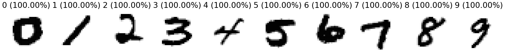
These are definitely more varied in style than the images the linear model was confident in.
Let’s train some images to optimize the model’s confidence:
examples = []
for digit in range(10):
    example = torch.full((28*28,), 0.5).requires_grad_()
    lr = 1
    conf = 0
    its = 0
    while conf < 0.9999:
        c = torch.softmax(simple_net.forward(example), dim=0)[digit]
        conf = c.item()
        torch.log(c).backward()
        example.data += example.grad * lr
        example.grad.zero_()
        example.data = torch.maximum(torch.minimum(example.data, torch.tensor(1)), torch.tensor(0))
        its += 1
    examples.append(example.view((28,28)))
show_images(examples)
lr = 1
These are… a complete disaster.
What of the adversarial examples, clamped close to a training 0? Here’s what we get with the same ±0.25 threshold:
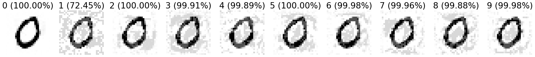
That threshold gives enough leeway to completely overwhelm the model’s predictions for all except the digit 1, and even then we can get the model to consider 1 unambiguously the most likely prediction. Clamping to ±0.125 is a more interesting threshold:
My unsurprising, albeit tentative, takeaway is that a two-layer neural net already behaves a lot more weirdly and is more resistant to interpretation than a one-layer one. (It also overfit a little — its accuracy was noticeably lower on the test set than the training set.)
Incidentally, comparing the last two images made me wonder — perhaps our adversarial example thresholds should be gamma-aware? This is left as an exercise to the reader.
Conclusion
Even the incredibly simple neural networks I built in this post behaved surprisingly and were more difficult to interpret than I expected. This left me rather ambivalent: on one hand, it’s great that there’s so much to explore and I never felt like I ran out of things to try even with minimal access to compute; but on the other, if even a 7,000-parameter model is so confusing, how on earth are we going to understand cutting-edge models with hundreds of billions of parameters?
Speaking purely about just the coding experience, it showed me pitfalls and taught me lessons about ML implementation that I thought would only arise at much larger scales and training times. One post I had been pointed to that described how ML engineering differed from other software was Lessons Learned Reproducing a Deep Reinforcement Learning Paper. Having read this post much earlier, I think I was inspired to “notice confusion” more often, which I think helped me avoid some (but not enough) bugs; but a different suggestion I wrongly thought I could get by without was:
For any project this long, detailed records of what you’ve tried and the ability to reproduce past experiments are an absolute must. Version control software can help, but a) managing large outputs can be painful, and b) requires extreme diligence. (For example, if you’ve set off some runs, then make a small change and launch another run, when you commit the results of the first runs, is it going to be clear which code was used?)
Even though my project were nowhere as long, my simple experiments
were already an absolute mess. The direst example was how I allowed
/255 to haphazardly drift through versions of my code and
wreak havoc. Still, overall I think I certainly have a little more
intuition and confidence about ML engineering now.
At the same time, given the apparent universality of these struggles, I can’t help but wonder if there’s still a lot of room for improving the basic languages and tools for architecting neural networks. Maybe writing ML code today is like managing memory with C — you can do it, but most human programmers will experience a lot of foot-shooting on the way, and there are abstractions that can fix all this, but they hadn’t been invented or popularized yet.
In any case, I learned a lot from writing this post and from the safety course. Thanks to the organizers and those in my cohort, and if any of my readers not from the program think the field is interesting, I’d suggest checking it out (though it’s very different from the things I covered in this post).