Just Enough Elliptic Curves to Be Dangerous

A famous Trail of Bits post says to stop using RSA: it’s simple enough to make people think they can implement it correctly, but full of invisible traps. In contrast, although elliptic curve cryptography (ECC) implementations could also fall into subtle traps, they usually don’t. The post conjectures that this is because ECC intimidates people into using cryptographically sound libraries instead of implementing their own.

If you do want to understand ECC just enough to produce your own trap-ridden implementation, though, this post aims to get you there. (Assuming some mathematical background chosen in a not particularly principled way, approximately what I had before writing this post.) Hence the title. Because I have a cryptographic conscience, I will still point out the traps I know of; but there are probably traps I don’t know about.

This post contains a lot of handwaving and straight-up giving up on proofs. You don’t need to know the proofs to be dangerous. The ethos is sort of like Napkin, but way shoddier and with zero pretense of pedagogical soundness. Still, here are some concrete questions that I learned the answer to while writing this post:

• Why does the group law hold, sort of intuitively?
• Why do people have to modify Curve25519 before using it to compute digital signatures?
• What is a “quadratic twist” and why should I care about it to pick a secure elliptic curve?
• How is it possible that an isogeny can be described as surjective but not injective while mapping a finite elliptic curve to another elliptic curve of the same cardinality?
• How many claws does an alligator have?

Elliptic curves have a lot of complicated algebra. If you ever studied algebra in high school and did exercises where you had to simplify or factor or graph some really complicated algebraic expression, and you learned that algebra is also the name of a field in higher mathematics, you might have assumed that working algebraists just dealt with even more complicated expressions. If you then studied algebra in college, you’d probably have realized that that’s not really what algebra is about at all; the difficulty comes from new abstractions, like a bunch of the terms above.

Well… the study of elliptic curves involves a bunch of complicated expressions like what your high school self might have imagined. Sometimes, notes will just explode into a trainwreck of terms like

\[\begin{align*}\psi_1 &= 1 \\ \psi_2 &= 2y \\ \psi_3 &= 3x^4 + 6Ax^2 + 12Bx - A^2 \\ \psi_4 &= 4y(x^6 + 5Ax^4 + 20Bx^3 - 5A^2x^2 - 4ABx - A^3 - 8B^2).\end{align*}\]

“This is REAL Math, done by REAL Mathematicians,” one is tempted to quip. The Explicit-Formulas Database is a fun place to take a gander through. I will copy formulas into this post from time to time when there’s something about them I want to call attention to, but in general we won’t do any complicated algebraic manipulations in this post. Just be prepared.

Because I’m focusing on conceptual understanding (and am lazy), this post contains almost no code, and definitely no code that’s runnable in any real programming language.

Background

To understand all of this post, you’ll need to be comfortable with quite a few things. The first and most obvious is basic modular arithmetic; if you’re not, I don’t have a resource to suggest offhand, but there’s “not that much” and the Wikipedia article is probably an okay starting point. I go over some of the slightly more advanced facts in the first subsection below.

You’ll also probably want to know basic abstract algebra: groups, rings, fields, and particularly \(\mathbb{F}_p\). Linear algebra is probably required too. (Amusingly, I believe you don’t need to know anything about the rationals \(\mathbb{Q}\), the reals \(\mathbb{R}\), or the complex numbers \(\mathbb{C}\). Everything is finite in our world.) If this is all new to you, you may be able to get some of these prerequisites from Napkin, but the prerequisites don’t have a neat shape. If you have learned these things before but it’s been a long time, the second subsection below has a speedy recap.

You should also feel free to skip this entire section and come back to it on a need-to-know basis. I know I would.

Background: Modular arithmetic, quadratic residues, and square roots

We will be working in \(\mathbb{F}_p\), that is in the field of integers modulo some prime \(p\), very often, so let’s quickly review some facts. The key things to understand here are (1) what happens to quadratic residues and quadratic nonresidues when they’re multiplied and (2) that square roots can be computed mod \(p\), so if you understand those you can skip this section. In finite fields of the form \(\mathbb{F}_p\),

• Inverses exist: for every nonzero \(a \in \mathbb{F}_p\), there exists \(b\) such that \(ab = 1\).
• (Fermat’s little theorem:) for every nonzero \(a \in \mathbb{F}_p\), \(a^{p-1} = 1\). The smallest positive integer \(m\) such that \(a^m = 1\) is called the order of \(a\); it follows that \(m\) divides \(p - 1\).
• The multiplicative group \(\mathbb{F}_p^\times\) is cyclic; that is, there exists an element \(g\) (sometimes called a primitive root) such that \(\{g^x \mid x \in \{0, \ldots, p-1\}\}\) is the set of all nonzero elements of \(\mathbb{F}_p\).
• If an element \(x \in \mathbb{F}_p\) is a square of some element, it is called a quadratic residue; otherwise, it is a quadratic nonresidue.
• If \(p > 2\), then for every nonzero \(a \in \mathbb{F}_p\), we have \(a^{\frac{p-1}{2}} \in \{-1, 1\}\). Furthermore, \(a^{\frac{p-1}{2}} = 1\) iff \(a\) is a quadratic residue. As corollaries:
  • The product of two quadratic residues is a quadratic residue.
  • The product of a quadratic residue and a quadratic nonresidue is a quadratic nonresidue.
  • The product of two quadratic nonresidues is a quadratic residue.
  • The inverse of a quadratic residue is a quadratic residue; the inverse of a quadratic nonresidue is a quadratic nonresidue.
• If \(p > 2\), exactly half of the \(p - 1\) nonzero elements of \(\mathbb{F}_p\) are quadratic residues.

Now let’s consider how to compute a square root of a quadratic residue modulo a prime \(p > 2\). (I believe what follows is the “Tonelli-Shanks algorithm”. It’s not the most efficient known algorithm, but it’s good enough for our purposes.)

Write \(p - 1 = s \cdot 2^r\) where \(s\) is odd (we’ll have \(r \geq 1\) since \(p\) is odd), and say we have \(a\) that we know is a quadratic residue mod \(p\) and want to compute a square root.

• If \(r = 1\) (i.e. \(p = 2s + 1\), \(p \equiv 3 \bmod 4\)), this is really easy: \(b := a^{\frac{s+1}{2}}\) works.

• If not, it’s still a good candidate because \(b^2 = a^{s+1}\) is a factor of \(a^s\) off, but \(a^{s\cdot 2^r} = 1\), so \(a^s\) has order dividing \(2^r\). In fact, since \(a\) is a quadratic residue, \(a^s\) is as well, and it has order dividing \(2^{r-1}\). Intuitively that means there’s a \(1/2^{r-1}\) “probability” that \(b\) is correct anyway, and if not we’ve reduced the problem of finding a square root of \(a\) to finding a square root of this low-order element \(a^s\).

  To handle this simpler problem, let \(u\) be an element with order \(2^r\). (This can be computed from any quadratic nonresidue \(t\): just set \(u = t^s\), and you can find a quadratic nonresidue by just randomly picking elements in \(\mathbb{F}_p\) until you find one; half the elements are quadratic nonresidues, so you should find one quickly. Not having reasonable worst-case bounds might still be moderately dissatisfying, but you can also precompute \(u\) or \(t\) for any given \(p\) so it’s not a big deal. There are specific applications where this still isn’t good enough, but they’re rare.)

  Then the square root of \(a^s\) is a power of \(u\). More explicitly, there is some \(k\) such that \(u^{2k} = a^s\), and we want to find \(u^k\). In particular, if \(r = 2\), then \(u\) is actually a square root of \(a^s\), and we’re done. Even in the general case, we can determine \(k\) bit by bit as follows: multiply \(a^s\) by \(u^{2^j}\) for increasing \(j\) and see if it decreases the order of \(a^s\).

Background: Abstract algebra speedrun

This is just a refresher, not an attempt to teach you these things! A lot of this section is written extremely technically imprecisely.

• An abelian group is a set where you can add and subtract: that is, a set equipped with an addition operation \((+)\) that has an identity (called the zero) and is associative, commutative, and invertible. (Groups, without the “abelian” adjective, differ only in that they lack the commutativity property.)

  • One can prove that all finite abelian groups are (isomorphic to) products of cyclic groups \(\mathbb{Z}/n\mathbb{Z}\) (integers modulo \(n\) under addition): that is, each element is a tuple of elements from those groups, and all operations happen componentwise. It’s possible to be even more precise, but that’s not super necessary.

• A ring is a set where you can add, subtract, and multiply, but where multiplication might be noncommutative: that is, a set equipped with an addition operation \((+)\) and zero and a multiplication operation \((\cdot)\) and one, such that the field is an abelian group under addition and zero, multiplication is associative and has one as an identity, and the distributive law holds.

• A field is a ring where multiplication is commutative and you can divide: that is, a ring where the nonzero elements of the field form an abelian group under multiplication and one.

• In vague terms, a “structure-preserving map” is a function \(\phi : A \to B\) between two “things” (e.g. groups, rings, vector spaces) \(A, B\) of the same kind, such that any operation (e.g. \(+\)) or special elements (e.g. \(0\)) are preserved by the map: \(\phi(a + b) = \phi(a) + \phi(b)\), \(\phi(0_A) = 0_B\), and so on. Note that \(\phi\) need not be injective or surjective.

  • A structure-preserving map on most algebraic structures, in particular groups, is a homomorphism.
  • A structure-preserving map from a structure to itself is an endomorphism.
  • A structure-preserving map with an inverse that’s also structure-preserving (implying that both are bijections) is an isomorphism. (Frequently, isomorphic things are considered “the same”.)
  • An endomorphism that’s an isomorphism is an automorphism.
  • The kernel of a structure-preserving map is the set of things it maps to \(0\).

• In vague terms, you can consider an algebraic structure \(X\) “modulo” some substructure or operation by considering things related by the substructure or operation as “the same”. More formally, you create a new algebraic structure \(X'\) whose elements are equivalence classes of \(X\) under some equivalence relation and inherits the same algebraic operations. Of course, a lot of conditions are required for the inherited operation to be well-defined.

  • (Aside: A “normal subgroup” of a group is a subset that’s itself a group and that you can mod by. An “ideal” of a ring is a subset that’s itself a ring and that you can mod by. These terms aren’t defined in any textbook this way, but I think they’re the “morally correct” ways to think about these concepts.)
  • (Aside 2: “modulo” is written with a slash \(/\) and is exactly the slash in the \(\mathbb{Z}/n\mathbb{Z}\) notation for “integers modulo \(n\) under addition”. \(n\mathbb{Z}\) is just the set of all multiples of \(n\), and if you take the integers and say “consider the set of all multiples of \(n\) the same”, you get integers modulo \(n\).)

• The substructure generated by some set of elements in a structure is the set of elements you can get by repeatedly applying the structure’s operations to only that set. For example, the subgroup generated by \(\{3\}\) in \(\mathbb{Z}/12\mathbb{Z}\) is \(\{0, 3, 6, 9\}\); those are the numbers you can get by repeatedly adding 3 to itself mod 12.

• The characteristic of a field \(\text{char}(\mathbb{K})\) is the number of times you add one to itself to get back to zero, or zero if that never happens. You can prove that the characteristic is always zero or a prime.¹

  Basically, the characteristic of \(\mathbb{Q}\), \(\mathbb{R}\), and \(\mathbb{C}\) are all 0, and the characteristic of \(\mathbb{F}_p\), \(\mathbb{F}_{p^k}\), \(\overline{\mathbb{F}_p}\) are all \(p\). In full generality, all fields contain either \(\mathbb{Q}\) or \(\mathbb{F}_p\) (just look at the subfield generated by 1) and that determines the characteristic.

• The algebraic closure of a field \(\mathbb{K}\), denoted \(\overline{\mathbb{K}}\), is the field extension (basically just a larger field) you get by adding all the roots of every (nontrivial) polynomial with coefficients in \(\mathbb{K}\). (It is unique up to isomorphism.) The most familiar example is that \(\mathbb{C}\) is the algebraic closure of \(\mathbb{R}\).

• Finally, one important algorithm: the repeated doubling algorithm lets you “multiply” a “thing” \(x\) by a positive integer \(n\) if you only know how to add, in \(O(\log n)\) additions. In a nutshell, you compute it recursively as \(A(x, 2n) = A(x, n) + A(x, n)\) and \(A(x, 2n+1) = A(x, 2n) + x\). You’ve probably done this if you’ve ever implemented modular exponentiation in a programming competition. We will use this in a few places for other kinds of “multiplication”. (There are ways to optimize the constant factors in this algorithm even more, but we won’t concern ourselves with them.)

Definition of an elliptic curve

With all that out of the way, let’s get started!

An elliptic curve over a field \(\mathbb{K}\) is a smooth projective curve of genus 1 with a distinguished (\(\mathbb{K}\)-rational) point.

This is a lot of words. Let’s break it down.

• The projective plane \(\mathbb{P}^2(\mathbb{K})\) over a field \(\mathbb{K}\) can be tersely defined as the set of nonzero three-dimensional points \((x : y : z)\) (where \(x, y, z \in \mathbb{K}\)) modulo scaling (i.e. for any \(\lambda \neq 0\), \((x : y : z)\) is the same point as \((\lambda x : \lambda y : \lambda z)\). The next section is about ways to view it.
• A curve is given by a homogeneous polynomial function \(f(x, y, z)\) that is irreducible (can’t be factored) even over \(\overline{\mathbb{K}}\) (!), and can be viewed as the set of points where that polynomial evaluates to 0. The polynomial is required to be homogeneous (all terms are the same degree, where the degree of a term is the total of the degrees of \(x\), \(y\), and \(z\)) so that this evaluation is well-defined on points modulo scaling, and is required to be irreducible so that the curve doesn’t turn out to be secretly two curves in a trenchcoat. (As an example, \(x^2 + 2y^2\) (the equation \(x^2 + 2y^2 = 0\)) is not a curve over \(\mathbb{R}\) even though it’s irreducible there, because it is reducible in \(\mathbb{C}\).)
• A curve is smooth if its three partial derivatives are never all zero. This matches the intuitive geometric meaning of the word “smooth” if the field is \(\mathbb{R}\); we just generalize it naively to all fields.
• Genus one means… honestly, I’m not really sure. I’m told it matches the topological definition of “number of holes in a sphere” (a sphere has genus 0, a torus has genus 1…) but I don’t know how many holes anything has in four dimensions (two complex dimensions). I’m going to leave this as “we’ll handwave it when we see it”.
• A distinguished point just means the point is part of the definition. If you have two copies of the same curve or polynomial, but distinguish different points on them, you get two different elliptic curves.

The projective plane

“Lines that are parallel
meet at Infinity!”
Euclid repeatedly,
heatedly,
    urged.
Until he died,
and so reached that vicinity:
in it he
found that the damned things diverged.

— Piet Hein, Grooks VI

In terms of why the projective plane \(\mathbb{P}^2(\mathbb{K})\) is worth studying, its most defining property is that every pair of lines intersects at exactly one point. (The dual, through every pair of points there is exactly one line, is still true, just like it is in Euclidean spaces.) In other words, there are no “parallel” lines. There are a few equivalent ways to understand or visualize the projective plane (in contrast to the Euclidean plane \(\mathbb{K}^2\), which may also be called the affine plane when directly contrasting the two):

• One can view it as an extension of the Euclidean plane: to such a plane, add a point at infinity for every “direction” (a direction is an equivalence class of parallel lines, so directions are the same as their opposites) and a single line at infinity that passes through precisely the set of points at infinity. A line in the Euclidean plane passes through exactly one point at infinity, the one matching its direction. Although the special cases are sort of inelegant, this view is nice in that it lets us think about (and compute!) two coordinates instead of three.
• Another way to view it is as the (two-dimensional) surface of a (three-dimensional) sphere, where lines are great circles (which are in fact the shortest paths between two points) and antipodes are considered the same point.

The terse definition we gave earlier turns out to be the easiest way to talk about the projective plane concretely with coordinates, though, which is important to analyze it algebraically. To repeat a bit, a projective point is a triplet of coordinates \((x : y : z)\), not all zero, modulo scaling: that is, if \(\lambda \neq 0\), then \((x : y : z)\) is the same point as \((\lambda x : \lambda y : \lambda z)\). One can visualize a projective “point” as a line in three-dimensional Euclidean space that passes through the origin, and a projective line as a plane that also passes through the origin. It’s also easy to relate this visualization back to the two earlier perspectives:

• To recover the Euclidean-plane-and-things-at-infinity view, just take the intersection of each line with the plane \(z = 1\); lines that intersect that plane correspond to that point on the plane; lines in the plane \(z = 0\) correspond to points at infinity, and the plane \(z = 0\) is the line at infinity. We will use this view extensively; when we write a projective point as \((x, y)\), it will be shorthand for \((x : y : 1)\), with the understanding that points at infinity cannot be represented this way.
• To recover the sphere view, just take the intersection of each line with a sphere centered at the origin.

Elliptic curves: the Weierstrass equation

Let \(\mathbb{K}\) be a field. It could be \(\mathbb{Q}\), \(\mathbb{R}\), \(\mathbb{C}\), a finite field \(\mathbb{F}_p\) or even \(\mathbb{F}_{p^k}\), and so on; but for our cryptographic purposes, \(\mathbb{K}\) will probably be \(\mathbb{F}_p\) for a large prime \(p\), typically close to \(2^{256}\). However, we will still have to care about the algebraic closure of \(\mathbb{F}_p\). (Occasionally, cryptography is done on a large characteristic-2 finite field \(\mathbb{F}_{2^k}\), but this is outside the scope of this post.)

Let \(\text{char}(\mathbb{K}) \neq 2, 3\) and let \(A, B \in \mathbb{K}\) with \(4A^3 + 27B^2 \neq 0\). (This is to avoid degenerate cases. A lot of theory still applies if \(\mathbb{K}\) is characteristic 2 or 3, but you sometimes end up with your hands tied unable to do some algebraic simplifications you really want to. It seems like a fair assumption for my motivations.) Then the (short) Weierstrass equation \(y^2 = x^3 + Ax + B\) with the distinguished projective point \((0 : 1 : 0)\) defines an elliptic curve.

(Beware! We will extensively write equations like this and pretend that the points on this elliptic curve are the pairs \((x, y)\) satisfying the equation in addition to that distinguished point, the point at infinity in the \(x = 0\) direction, which will sometimes just be denoted \(\infty\). However, the equation is “really” the homogeneous cubic \(y^2z = x^3 + Axz^2 + Bz^3\).)

Up to isomorphism, every elliptic curve can be defined this way! (This is not obvious. We haven’t even defined what an isomorphism is for our purposes.) For example, if you have an elliptic curve defined by \(y^2 = x^3 + Cx^2 + Ax + B\), you can substitute \(x = x' - C/3\) and get something absurd like:

\[y^2 = x'^3 + (A - C^2/3)x' + (B + 2C^3/27 - AC^3/3).\]

I don’t know if I got the later terms right, but the point is that this is a curve in Weierstrass form, and the simple bijection \((x, y) \mapsto (x + C/3, y)\) maps every point in the original curve to a point in this one. You can make similar substitutions to curve equations with more coefficients to get them into Weierstrass form. However, note that in the above example, we assume you can divide by 3; if you can’t because \(\text{char}(\mathbb{K})\) is 3, this doesn’t work, and similar problems arise if \(\text{char}(\mathbb{K})\) is 2, which is why we ban those cases above.

If you permit a few extra terms, you get a “general Weierstrass equation” that works for all fields, but I won’t bother here.

Other equations

Although short Weierstrass form is probably the most canonical way to write equations for elliptic curves to study them abstractly, there are other forms popular in cryptography. Particularly notable are Montgomery curves, which take the form \[By^2 = x^3 + Ax^2 + x.\]

Two also important alternative models of elliptic curves are Edwards curves of the form \[x^2 + y^2 = 1 + Dx^2y^2\] and slightly generalized twisted Edwards curves of the form \[Ax^2 + y^2 = 1 + Dx^2y^2.\] Which, just to be clear, is technically the homogeneous quartic \[Ax^2z^2 + y^2z^2 = z^4 + Dx^2y^2\] over the projective plane.

WARNING: Many sources gloss over this point, but Edwards curves and twisted Edwards curves are “not technically elliptic curves” because they are not smooth at their points at infinity (namely, \((1 : 0 : 0)\) and \((0 : 1 : 0)\))! They can be desingularized into the “curve” \[Ax^2 + y^2 = z^2 + Dt^2,\; xy = tz\] in the “projective space” \(\mathbb{P}^3(\mathbb{K})\) of 4-tuples \((x : y : z : t)\), not all zero, modulo scaling.² Tuples with \(z \neq 0\) can be scaled to affine points \((x : y : 1 : xy)\), which are in one-to-one correspondence with affine points \((x : y : 1)\) on the Edwards curve. However, this new curve has four points at infinity, \((\pm\sqrt{D/A} : 0 : 0 : 1)\) and \((0 : \pm\sqrt{D} : 0 : 1)\), instead of two. Note that \(\sqrt{D/A}\) and \(\sqrt{D}\) may not exist in whatever field \(\mathbb{K}\) we’re working over — in fact, we’ll later see that we prefer they don’t exist — but they definitely exist in the algebraic closure \(\overline{\mathbb{K}}\). Our definition doesn’t have any carve-out for curves specified by projective spaces with two equations, but most sources just handwave over this, so I will too.

A few famous curves

This section contains quite a few terms I haven’t defined yet, but I thought that getting to see the concrete objects we care about would be somewhat illuminating.

• NIST P-256 (NIST, 2000): One of several curves in that standard. \[y^2 = x^3-3x+B \bmod 2^{256} - 2^{224} + 2^{192} + 2^{96} - 1\] where \(B\) equals 41058363725152142129326129780047268409114441015993725554835256314039467401291. One of the earliest curves to be heavily standardized, but looked upon with some suspicion due to the unexplained large constant coefficient that might be a backdoor. It also predates modern EC cryptographic demands like Montgomery ladder support and twist security.
• secp256k1 (Certicom Research, 2000 (PDF); cr.yp.to ref): \[y^2 = x^3+7 \bmod {2^{256} - 2^{32} - 977}.\] One of several curves in that publication. Its claim to fame is probably being the curve used for signatures in Bitcoin. Although cryptographers aren’t concerned about a backdoor on this curve, it still fails some modern demands like P-256.
• Curve25519 (Bernstein, 2006): \[y^2 = x^3 + 486662x^2 + x \bmod {2^{255} - 19}.\] Chosen very carefully for efficiency, but without sacrificing any safety guarantees, including many discovered after 2000. Probably the vanguard of “modern curves”. Quite popular, although the original paper focuses on the Kummer variety of the curve rather than the curve itself, making it excellent for Diffie-Hellman but not a direct fit for more advanced algorithms. As a result, this is also often used in the form of its twisted Edwards curve, \[-x^2 + y^2 = 1 - \frac{121665}{121666}x^2y^2 \bmod {2^{255} - 19}.\]

The group operation and group law

I think most pop science explainers of elliptic curves already have nice pictures of this, so I’ll take it a bit more slowly.

Interesting fact: Over any given fixed field, a line that intersects an elliptic curve at least twice always intersects it at exactly three points, where points of tangency count double.

• Geometrically, this might be a bit surprising or hard to visualize. One simpler case that helped me be intuitively less surprised: a unit circle is a curve such that a line that intersects it once must intersect it twice, again counting points of tangency double.
• However, it’s very easy to prove algebraically: to find the intersections of an elliptic curve \(E\) and a line \(\ell\), you substitute the line’s equation into the elliptic curve’s equation to get a cubic in \(x\) and then count how many roots it has. If that cubic has two solutions in any given field, it has a third, because you can factor out the first two roots as linear factors to get a final linear factor.

We will now define addition of two points on the elliptic curve (a commutative group operation) to satisfy this short, punchy “functional equation”: three points on a line sum to zero. Wait, but what is zero? We define zero to be the distinguished point, usually called \(O\), our elliptic curve comes with. Maybe a less sequence-breaking way to say it is that we define group inverses to be such that the distinguished point is zero, i.e., the inverse of a point \(P\) is the third point that the line through \(P\) and \(O\) intersects the elliptic curve at, and then define addition so that the functional equation works out. (It’s not obvious that these definitions are coherent, but that’s what we’ll explore in the rest of this section.)

So, although the functional equation is punchy, the explicit group operation is a little more work to describe and goes like this: Let \(O\) be the distinguished point. To add two points \(P, Q\) on an elliptic curve:

• Draw the line through \(P\) and \(Q\) and let \(R\) be the third point where the line intersects the curve (which could equal \(P\) or \(Q\) in case of tangency, and could be the point at infinity).
• Draw the line through \(R\) and \(O\) and let \(R'\) be the third point where the line intersects the curve (same caveats).
• Then \(P + Q = R'\).

When the curve is in Weierstrass form, we will just about always choose the unique point at infinity on the elliptic curve, \((0 : 1 : 0)\), as our distinguished point. In that case, the middle part of the above description becomes a bit simpler: \(R'\), the negation of \(R\), is just the reflection of \(R\) about the \(x\)-axis. To actually implement this, you could work out all the algebra in the above description to produce formulas that you can put into your program, but in practice, you can just get them from the Explicit-Formulas Database. But I think it’s worth saying this explicitly: you could choose a random other distinguished point that isn’t the point at infinity and define addition and inverses around it, and the theory still works. Computation just gets waaaay more complicated.

Defined as such, it’s pretty obvious that addition is commutative and that inverses “work”. However, it is extremely nonobvious that addition is associative.

Proof the group operation is associative

Proof. (Playing fast and loose; a small variant ripped from 18.783 with a phantom point instead of a proof by contradiction)

Suppose we want to prove that \(P + (Q + R) = (P + Q) + R\). Consider the following diagram, where all labeled points are points on the elliptic curve.

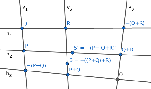
We want to prove that \(S = S'\). However, we will use a slight detour: we will define \(T\) to be the intersection of \(h_2\) and \(v_2\), and prove that \(T\) lies on the elliptic curve, from which we will have \(S = T = S'\).

Intuitively we’ll find that, because these nine points are the intersections of two triplets of lines, evaluating to zero at them are “linearly dependent” events, and that \(f\) being zero at eight of them will imply that it’s also zero at the ninth.

More rigorously:

• Consider the vector space of degree-3 homogeneous polynomials in \(x, y, z\). One can count that there are 10 distinct cubic terms in three variables:

  x³  x²y xy²  y³
    x²z xyz y²z
      xz² yz²
        z³

  Every such polynomial is a linear combination of these terms and only these terms, so this vector space has dimension 10.

• Consider the subspace \(V\) of degree-3 homogeneous polynomials that are zero at the eight labeled points other than \(S\) and \(S'\). Each restriction reduces the dimension by 1, so this subspace has dimension 2. (This is not true in general, but it’s “usually” true. In particular, it’s true if we assume the points are in general position and there are no “weird collinearities”. You can prove it if you can construct, for each of the eight points, a polynomial that’s nonzero at that point and zero at the seven others.)
• The elliptic curve \(f\) is in \(V\).
• Multiply the “horizontal lines” \(h_1, h_2, h_3\) to get a polynomial \(g(x, y, z)\): this is a degree-3 homogeneous polynomial that is zero at the eight points above, so it’s in \(V\). Also, \(g(T) = 0\).
• Multiply the “vertical lines” \(v_1, v_2, v_3\) to get a polynomial \(h(x, y, z)\): this is a degree-3 homogeneous polynomial that is zero at the eight points above, so it’s in \(V\). Also, \(h(T) = 0\).

• Because the three polynomials \(f, g, h\) are all in this dimension-2 subspace, they must be linearly dependent. \(g\) and \(h\) are not multiples of each other (they have different factors), so \(f\) must participate in this linear dependence. By evaluating this linear dependence at \(T\), we conclude that \(f(T) = 0\), i.e., \(T\) is on the elliptic curve. Therefore, \(S = T = S'\), and we’re done.

This proves the addition we defined is associative in the general case, where there are no “weird collinearities”. I feel like you should be able to generalize it to arbitrary points just by handwaving it as: you can expand out associativity as a massive equation that’s still purely algebraic and finite degree; the above proof shows that this equation is true almost everywhere, so it must be true everywhere, because polynomials can’t have that many zeros. But nobody seems to be willing to do this, so maybe this doesn’t work or is more annoying than bashing it from other angles. Regardless, I think this gets the intuition across pretty well.

Entering the danger zone: Elliptic Curve Diffie-Hellman

Understanding the group operation is basically all you need to do to do elliptic curve cryptography dangerously. Here’s the simplest ECC protocol, an elliptic-curve Diffie-Hellman exchange, between Alice and Bob:

• They agree on an elliptic curve \(E\) and a point \(P\) that generates a subgroup \(G\). This can be done completely publicly and predictably, most likely hardcoded into the software Alice and Bob are using, using parameters plucked off an RFC (a kind of Internet standard). Suppose \(G\) has size \(n\).
• Alice and Bob each generate a secret integer, respectively \(a\) and \(b\), in the range \(0 < a, b < n\).
• Alice and Bob compute and publish the result of scalar multiplication of \(P\) with their integers; that is, Alice computes \(P + P + \cdots + P\), applying the group operation to \(a\) copies of \(P\) (but actually computing it with repeated doubling so it runs in a reasonable time), and similarly for Bob. The whimsical but standard notation we’ll use for scalar multiplication is \([a](P) = P + \cdots + P\), where there are \(a\) copies of \(P\) (or \(|n|\) copies of \(-P\) if \(n < 0\)); so Alice publishes \([a](P)\) and Bob publishes \([b](P)\).
• Alice computes \([a]([b](P))\) and Bob computes \([b]([a](P))\). Both equal \([ab](P)\), and they can use that as their shared secret.
• However, an adversary sees only \([a](P)\) and \([b](P)\) (and \(P\) itself). As far as we know, there is no general practical algorithm to compute \([ab](P)\) from this information. (This is called the computational Diffie-Hellman assumption for an elliptic curve group; many cryptosystems are proven secure under it. Sometimes the stronger decisional Diffie-Hellman assumption is also invoked.)
  • (Both assumptions are stronger than the assumption that discrete logarithms are hard to compute. Computing a discrete logarithm just means, given \(P\) and \([a](P)\), computing \(a\); and of course if the adversary could do that, they could completely break the cryptosystem we’re describing.)
• Alice and Bob can now communicate with a much cheaper symmetric encryption system seeded with that shared key, \([ab](P)\), that no eavesdropper can derive.

Of course, to implement even this simple protocol, you have to actually write down formulas for point addition, which can be quite painful. You can get them from — wait for it — the Explicit-Formulas Database, so I won’t go into them here.

Although this cryptosystem is secure at a high level, there’s already (at least) three broad categories of traps and vulnerabilities one can fall prey to when trying to implement it.

1. The theoretical trap: small subgroup attacks
2. The implementation trap: timing side channels
3. The hybrid trap: invalid curve attacks

So here’s the cryptographic conscience part of this post.

(I mostly just ripped this from SafeCurves. One attack I won’t delve into is the transfer, both because I don’t understand it and because, unlike these other traps, it seems to be difficult to make your curve vulnerable to a transfer unless you’re explicitly trying. I believe transfers might be useful for carrying out an invalid curve attack, but I won’t go into that.)

Theoretical trap: small subgroup attacks

The theoretical trap is that we really want \(n\), the size of the group \(G\), to be a large prime. If \(n\) is the product of small primes, then you can practically compute \(a\) from \([a](P)\) by computing it modulo each small prime and then combining the results with the Chinese Remainder Theorem. Even if \(n\) is, say, 2 times a large prime, \([a](P)\) still leaks the lower bit of \(a\), which we’d rather avoid.

However, for other reasons we’ll mention later, there are other properties we want \(E\) to have that, as a side effect, make it impossible for the size of \(E\) to be a large prime. So we typically compromise by choosing \(E\) such that its size is a small integer \(h\) times a large prime \(\ell\), and then take \(G\) to be a proper subgroup of size \(\ell\) (well, the proper subgroup). The integer \(h\) is called the cofactor. As an example, Curve25519 (the Montgomery curve \(y^2 = x^3 + 486662x^2 + x\) over \(\mathbb{F}_{2^{255} - 19}\)) has size \(8\ell\), where \[\ell = 2^{252} + 27742317777372353535851937790883648493\] is prime; its cofactor is \(8\).

While you can avoid leaking the lower bits of private keys on such a curve by choosing \(P\) to be a generator of \(G\) instead of the entirety of \(E\), this is risky. If Alice is doing a DH key exchange with Bob, Bob could maliciously send Alice a point outside \(G\) (i.e. that isn’t a multiple of \(P\)) in the second step to leak Alice’s private key’s lower bits. Alice can check that Bob’s point is in \(G\) before responding, but this is both computationally expensive and an extra implementation footgun. (You might say that leaking a few bits of a secret key isn’t a big deal since you still have about 250 remaining bits of entropy, and you might be right for the simple Diffie-Hellman exchanges we’re considering, but this leak can actually be catastrophic for other protocols.³) Curve25519 sidesteps this issue more deeply by keeping \(P\) as a generator of the full group \(E\), but tweaking the protocol by asserting that private keys must be chosen to be multiples of 8, so there are no lower bits to leak.

There are more complicated use cases for elliptic curves where this compromise still isn’t good enough, and cryptographers have developed more advanced techniques for getting a prime-order group out of an elliptic curve with a small cofactor. That is, they’ve designed an abstraction of elements, built atop the elliptic curve, that behave and can be manipulated exactly like “elements of a prime-order group”, while keeping comparable efficiency and obviating any validity checks. Decaf (Hamburg 2015) is a technique for getting a prime-order group out of an elliptic curve with cofactor 4; Ristretto is a similar technique for elliptic curves with cofactor 8. Both links also discuss the pitfalls of using elliptic curves with cofactors or trying to hack around the cofactor with simple fixes in more depth. Unfortunately, exactly how they work is beyond the scope of this post.

Implementation trap: timing side channels

The implementation trap is that naïve repeated doubling leaks information about \(a\) and \(b\) through timing. The “repeated doubling” algorithm I described way at the start of this post might be written something like:

def repeated_doubling(n, P):
    if n == 0: return 0 # as an EC point
    if n % 2 == 0:
        Q = repeated_doubling(n // 2, P)
        return Q + Q # in the EC group
    else:
        return repeated_doubling(n - 1, P) + P # in the EC group

This takes longer when \(n\) is larger or has more 1’s in their binary representations, which is undesirable. A standard constant-time algorithm to compute \([n](P)\), where \(0 \leq n < 2^m\) for some fixed public \(m\), is the Montgomery ladder, which runs as follows in pseudo-Python:

def montgomery_ladder(n, P):
    "Computes [n](P) in constant time, given that 0 <= n < 2^m"

    r0 = 0 # as an EC point
    r1 = P # as an EC point
    for i in range(m - 1, -1, -1): # m - 1 to 0 inclusive
        if ((n >> i) & 1) != 0:
            r1 = r0 + r1 # in the EC group
            r0 = r0 + r0 # in the EC group; doubling
        else:
            r0 = r0 + r1 # in the EC group
            r1 = r1 + r1 # in the EC group; doubling

        # Invariant: At this point, r0 = [(n >> i)](P), r1 = [(n >> i)+1](P)
    return r0

(The Montgomery ladder may also refer to a more specific version of this algorithm optimized for Montgomery curves, which we’ll talk about in a few sections.)

There are many elliptic curves where doubling a point can be done faster than adding two points, but still in constant time; in those cases you can replace the two doubling lines with that instead without affecting the timing security. Of course, all this assumes that adding two points is a constant-time operation and that the branch on private data doesn’t leak through a side channel more sophisticated than raw timing, but you can avoid those leaks with standard techniques relatively straightforwardly and cheaply; the overhead would still be dwarfed by performing the actual elliptic point additions.

Hybrid trap: invalid curve attacks

The last trap I want to talk about falls somewhere in between the above cases. What if, during a DH key exchange, Bob gives Alice a maliciously crafted point \(P\) that isn’t on the curve at all?

Of course, Alice can explicitly plug Bob’s point into the elliptic curve equation and error out if it’s not satisfied, but it’s worth thinking about what might go wrong if Alice forgets to do this. This attack can’t really be discussed in full generality because it depends on exactly what algorithm or formula Alice is using to compute scalar multiplications of elliptic curve points, and we’ll revisit it in later sections; but for now, let’s pretend this DH key exchange is taking place on a short Weierstrass form elliptic curve with the formulas taken directly from the Explicit-Formulas database.

Well, I copied over the formulas: for the curve \(y^2 = x^3 + Ax + B\), the addition of two affine points \((x_1, y_1) + (x_2, y_2)\) is \[\left( \frac{(y_2 - y_1)^2}{(x_2 - x_1)^2} - x_1 - x_2, \frac{(2x_1 + x_2)(y_2 - y_1)}{x_2 - x_1} - \frac{(y^2 - y_1)^3}{(x_2 - x_1)^3} - y_1 \right),\] while the doubling of an affine point \((x, y)\) is \[\left( \frac{(3x^2 + A)^2}{4y^2} - 2x, \frac{3x(3x^2 + A)}{2y} - \frac{(3x^2+A)^3}{8y^3} - y \right).\] You do not need to understand these formulas. There’s only one thing you need to observe about them: they don’t depend on \(B\). This means that, if Bob gives Alice a malicious point \((x, y)\) lying on another curve of the form \(y^2 = x^3 + Ax + B'\) for some \(B'\) (and in fact it’s easy to see that every point \((x, y)\) lies on exactly one curve of that form), and if Alice blithely shoves them into the above formulas, then Alice will unwittingly be computing scalar multiplication on that curve instead! And if Bob picks \((x, y)\) such that it generates a subgroup with small or smooth order of its curve, which typically isn’t hard since he has so much freedom, he can leak Alice’s private key by examining the result.

The obvious takeaway is that, when Alice performs a Diffie-Hellman key exchange, she needs to validate that the point she gets is on the curve she expects it to be. However, we’ll soon see other ways to choose and implement elliptic curves that prevent this attack more fundamentally. Letting implementors skip this check is not just good in that it removes a footgun, it can also make implementations more efficient.

The x-only optimization and the Montgomery ladder

There are a variety of ways to optimize elliptic curve optimizations beyond just plugging \(x\) and \(y\) coordinates into formulas and performing modular arithmetic. For example, you might represent \(x\) with two numbers \(x'\) and \(z'\), where \(x = x'/z' \bmod{p}\), so that when you want to divide \(x\) by a number, instead multiply \(z'\) by it. This lets you minimize the number of division operations (which are computationally much more expensive than multiplications). Occasionally, a more complicated representation like \(x = x'/z'^2\) is better. There are many variants depending on the curve type, so I won’t go into details (I don’t understand all of them anyway).

However, I will just focus on one of the most interesting optimizations, which doubles as a partial mitigation of invalid curve attacks: tracking only the \(x\)-coordinate of a point on the elliptic curve. This makes sense since, given that a point is on the elliptic curve and you know its \(x\)-coordinate, its \(y\)-coordinate is almost entirely redundant, but not quite: from a theoretical standpoint, dropping it is equivalent to taking points of the elliptic curve modulo negation. (The resulting mathematical object is apparently called the Kummer variety of the elliptic curve, although not a lot of sources bother to name it as such.) It should be surprising that this works because it isn’t a traditionally valid kind of “modulo”, since it causes the group operation to no longer be well-defined: \(P + Q\) and \(P + (-Q)\) do not have the same \(x\)-coordinate in general, even though their operands do. However, scalar multiplication is still well-defined, and that is enough for Diffie-Hellman.

What’s more, Montgomery curves (those of the form \(By^2 = x^3 + Ax^2 + x\)) in particular have the following property: if you have the \(x\)-coordinate of the three points \(A\), \(B\), and \(A - B\), you can quickly compute the \(x\)-coordinate of \(A + B\). And this assumption is true for every addition in the Montgomery ladder above! As a result, scalar multiplications can be computed particularly quickly on Montgomery curves.

(Every Montgomery curve’s order is even, which you can see just from the fact that \((0, 0)\) is on every such curve, and that point doubles to \(\infty\). In fact, every Montgomery curve’s order is divisible by \(4\). The computational advantages are so great that they outweigh our earlier desire for \(E\) to be of prime order and motivate us to settle for a cofactor.)

You can find derivations of the formulas in Montgomery curves and the Montgomery ladder (Bernstein and Lange, 2017). One particular caveat to be aware of is that these ladders conflate the \((0, 0)\) point with the point at infinity, and assigns the \(x\) coordinate of 0 to both. This optimization is very much enshrined in the definition of Curve25519 (PDF). Public keys represent equivalence classes of a point and its negation; the “base point” \(P\) is the pair of points that have \(x = 9\).

As I mentioned briefly, this also greatly reduces the attack surface for invalid curve attacks. The formulas in the Montgomery ladder also don’t depend on \(B\); however, for fixed \(A\) in the Montgomery equation \(By^2 = x^3 + Ax^2 + x\), there are only two Montgomery curves up to isomorphism.

• If \(B'/B\) is a quadratic residue, then there is an obvious isomorphism between \(By^2 = x^3 + Ax^2 + x\) and \(B'y^2 = x^3 + Ax^2 + x\), namely \((x, y) \mapsto (x, y/\sqrt{B/B'})\).
• Otherwise (since \(B' = 0\) obviously doesn’t produce a curve) exactly one of \(B\) and \(B'\) is a quadratic residue, and all such values \(B'\) produce curves are isomorphic to each other. Any such curve is called the quadratic twist of the original curve.

(Note that, if you consider these curves over the field \(\overline{\mathbb{K}}\), in which \(\sqrt{B/B'}\) exists, then this distinction does not exist: any curves with the same \(A\) are isomorphic, which include any curve and its quadratic twist as we defined them above. In this way, you can view the curve and its quadratic twist as subgroups of a larger group, which have only the identity and a few other low-order points in common.)

Every \(x\)-coordinate that doesn’t represent a pair of points on a Montgomery curve represents a pair of points on its quadratic twist, and Curve25519 was chosen such that its quadratic twist’s order is 4 times a large prime. This means that if a malicious Bob sends Alice a number that isn’t the \(x\)-coordinate of any point on Curve25519, and Alice dutifully performs a scalar multiplication and reports the result to Bob, Bob still can’t make meaningful progress towards determining Alice’s private key. Either his point will be on the quadratic twist, on which the discrete log problem is just as hard, or it will be an extra useless point like 0.

While all this makes for really performant and secure DH, it also implies that you cannot directly perform group addition on two strings representing “points on Curve25519”; they actually represent points on the Kummer variety, or equivalence classes of two points on the elliptic curve; and addition on them isn’t well-defined. This is why (or, at least, it’s one of the reasons) Curve25519 as defined above is not directly used in other cryptographic protocols that require you to be able to add points, such as the Digital Signature Algorithm (DSA, or ECDSA if specifically instantiated with an elliptic curve). (This hasn’t stopped cryptographers from figuring out how to use Curve25519 to make signatures anyway, see e.g. qDSA, but it’s a bit trickier and beyond the scope of this post.)

Group operations on twisted Edwards curves

Fortunately, if we want to implement other protocols that require being able to add unrelated points, we can still take advantage of the work put into choosing the parameters of Curve25519 as follows. Every Montgomery form curve is birationally equivalent to a twisted Edwards curve (one of the form \(Ax^2 + y^2 = 1 + Dx^2y^2\)), which has very nice general group addition formulas. (Two curves are birationally equivalent if there are rational maps that bijectively send them to each other. We’ll define “rational maps” in the next section.) Specifically, Curve25519 is birationally equivalent to \[-x^2 + y^2 = 1 - \frac{121665}{121666}x^2y^2.\] To a pure mathematician, they might as well be “the same” mathematical object, but computationally they of course have quite different point representations and formulas.

One mapping from Curve25519 to this curve is \[(x, y) \mapsto \left(\sqrt{-486664}\frac{x}{y}, \frac{x-1}{x+1}\right).\] (You can pick either sign for \(\sqrt{-486664}\). To be clear, we could evaluate both \(121665/121666\) and \(\sqrt{-486664}\) to integers in \(\mathbb{F}_{2^{255}-19}\), but they would be huge and not illuminating.)

WARNING: You cannot plug every point \((x, y)\) on the Curve25519 Montgomery curve into this formula to map it onto the twisted Edwards curve given above. Some points will obviously lead to division by zero; there’s some discussion on StackExchange, What does “birational equivalence” mean in a cryptographic context?; this confusion has caused real crytographic bugs. Despite that, the rational map is defined everywhere and is a perfect bijection of the Curve25519 Montgomery curve and the twisted Edwards curve (well, its desingularization). This should be surprising, but it’s consistent for a rational map to be defined everywhere even though one particular way of writing it down as formulas isn’t.

To see what’s going on, let’s go back to explicitly writing projective points as triplets for a moment. This is the mapping given above written out as such: \[(x : y : z) \mapsto \left(\sqrt{-486664}\frac{x}{y} : \frac{x - z}{x + z} : 1\right).\] Evaluating this at \((0 : 0 : 1)\) leads to division by zero when computing \(x/y\). However, we know that \(x, y, z\) satisfy \(y^2z = x^3 + 486662x^2z + xz^2\), which can be formally rearranged as \[\frac{x}{y} = \frac{yz}{x^2 + 486662xyz + z^2}.\] Therefore, the rational map is the same rational map as \[(x, y, z) \mapsto \left(\sqrt{-486664}\frac{yz}{x^2 + 486662xyz + z^2}, \frac{x - z}{x + z}, 1\right),\] and this way of writing it down can be evaluated at \((0 : 0 : 1)\) to get \((0 : -1 : 1)\), which is the affine point \((0, -1)\), on the twisted Edwards curve.

Evaluating the mapping at the point at infinity \((0 : 1 : 0)\) is a little more work. This time we can formally rearrange the Curve25519 equation as \[\begin{align*} y^2z - 486660x^2z &= x^3 + 2x^2z + zx^2 \\ (y^2 - 486660x^2)z &= x(x + z)^2 \\ \frac{z}{x + z} &= \frac{x(x+z)}{y^2 - 486660x^2} \\ \frac{x - z}{x + z} &= 1 - 2\frac{z}{x+z} \\ &= 1 - 2\frac{x(x+z)}{y^2 - 486660x^2}. \\ \end{align*}\] Our rational map is thus the same rational map as \[(x : y : z) \mapsto \left(\sqrt{-486664}\frac{x}{y} : 1 - 2\frac{x(x+z)}{y^2 - 486660x^2} : 1\right),\] and this can be evaluated at \((0 : 1 : 0)\) to get \((0 : 1 : 1)\), the affine point \((0, 1)\) on the twisted Edwards curve.

The inverse mapping, from the Edwards curve to the Montgomery curve, is \[(x, y) \mapsto \left(\frac{1+y}{1-y}, \frac{\sqrt{486664}(1+y)}{x(1-y)}\right).\] This is similarly not defined everywhere.

Of course, in both cases it’s probably simplest if the code picks a simple representation of the mapping and handles the special cases separately.

Point representations and invalid curve attacks on twisted Edwards curves

Since twisted Edwards curves are so important, let’s take a little time to make sure we understand how to represent points and perform group operations on them. Unlike Weierstrass and Montgomery curves, where there’s a special point at infinity and where you might have discovered that the Explicit-Formulas Database lists some special cases you must check for when adding two points, Edwards curves have complete formulas, which are formulas that don’t have special cases of “if statements”. (ETA: Actually, the preceding sentence is not true any more; complete formulas have been developed for many of these other curves. But this is a relatively recent development from 2015–2017 or so.) They also don’t have points at infinity, so you can always represent every point as a pair of coordinates \((x, y)\) from whatever finite field you’re working over. The group identity is \((0, 1)\). This makes group operations on Edwards curves particularly easy to implement correctly without timing side channel leaks.

If you remember when I introduced twisted Edwards curves, you might have objected to the claim that Edwards curves don’t have points at infinity, so let me be more precise. If considered over the algebraic closure \(\overline{\mathbb{F}_{2^{255}-19}}\), the twisted Edwards curve we said was isomorphic to Curve25519 has the points at infinity \((\pm\sqrt{-121665/121666} : 0 : 0 : 1)\) and \((0 : \pm\sqrt{121665/121666} : 0 : 1)\). However, both numbers \(\pm 121665/121666\) are not quadratic residues in \(\mathbb{F}_{2^{255}-19}\), so these points at infinity don’t exist over \(\mathbb{F}_{2^{255}-19}\).

So what about invalid curve attacks in this new setting? The formulas for point addition on Edwards curves are that \((x_1, y_1) + (x_2, y_2)\) are \[\left(\frac{x_1y_2 + y_1x_2}{1 + dx_1x_2y_1y_2}, \frac{y_1y_2 - Ax_1x_2}{1 - dx_1x_2y_1y_2}\right).\] They use all of its coefficients, so it’s not obvious what happens if you try to carry out an invalid curve attack with two random coordinates that aren’t on the curve. But Neves and Tibouchi, 2015 point out that if you naively plug in points \((0, y_1)\) and \((0, y_2)\) into the above formulas, you get \((0, y_1y_2)\), which means your group operation degenerates into multiplication in \(\mathbb{F}_p\). The discrete log problem is much easier in that group, though not obviously so (I believe no general polynomial-time algorithm is known; the constants and rates of growth in the best exponential algorithms are just much smaller).

In a nutshell, invalid curve attacks are still a concern. This time, I am not aware of a cleverer fix than just validating that untrusted points are on the curves you expect them to be on.

Finding points on curves

This is a detour that’s only relevant for EC cryptographic algorithms that are even more complicated than ECDH or ECDSA, but it’s related to stuff that came up at work and I think it’s interesting.

Here is a surprisingly nontrivial problem: Given an elliptic curve — let’s say it’s provided in Weierstrass form \(y^2 = x^3 + Ax + B\) — construct a nontrivial point on it.

The easiest strategy is probably the following rejection sampling strategy: Choose random \(x\), check if \(x^3 + Ax + B\) is a quadratic residue, and if so, compute one of its square roots \(y\) and output \((x, y)\); otherwise, repeat. Sometimes, we want a deterministic strategy that generates a point from a seed, in which case we might modify the above strategy by deterministically deriving each candidate \(x\) from the seed, say by concatenating a positive integer and cryptographically hashing.

While this strategy is simple, for some cryptographic applications it has a fatal flaw: it isn’t constant time. So to refine our search criteria a little, we want a deterministic function \(f\) from a large domain \(D\) to an elliptic curve \(E\) satisfying these criteria:

1. It should be efficiently computable in constant time. We can modify the rejection sampling strategy into a function that’s efficient on average and can be made effectively constant time by just always sampling a high number of points, enough that the probability of all of them failing is negligible, and taking the first point that succeeds; but this makes it quite inefficient.
2. It should have large range. We don’t want a function that just maps every input to the same precomputed point.
3. Its output should not reveal its discrete logarithm with respect to any other point, because many protocols’ security depend on that being secret or unknown. This eliminates the simple strategy of precomputing a generator \(G\) of the elliptic curve and mapping \(n \mapsto G^n\), which is otherwise actually quite nice.
4. Preferably, it should be somewhat evenly distributed across the curve. Note that we won’t give a strict definition of what “evenly distributed” is.
5. Preferably, it should be efficiently invertible on its range: if we know that a point \(P\) is in the image of \(f\), we may want to be able to efficiently compute \(d \in D\) such that \(f(d) = P\). Sometimes we will use this property by repeatedly generating random \(P \in E\) until we find one in \(f\)’s image, and then outputting its inverse. This is also nonconstant time rejection sampling, but it turns out that in some use cases, this timing leak doesn’t leak anything we care about whereas the original timing leak does.

There are two applications I know of such a function:

1. Indistinguishability: Represent a point on an elliptic curve in a way such that an adversary can’t distinguish it from random data. I think the idea is that if your protocol sends undisguised points on elliptic curves, a censor who doesn’t want you to use public-key cryptography can notice that by checking that the data you’re sending satisfies an elliptic curve equation and punish you.
2. Hashing to curves: Given a string, hash it to produce a point on the elliptic curve in a way that has all the usual properties you’d want from a cryptographic hash. I won’t justify this in detail, but there are several protocols where this is a useful primitive.

Stated thus, the problem turns out to be important and difficult enough that it has led to multiple solutions with multiple names attached. Most of them are “convert the seed into an element of \(\mathbb{F_p}\) and plug it into these huge algebraic formulas”, but instead of telling you the formulas, I’ll just leave references to them and try to leave you with the motivation for coming up with those formulas, enough that you can reconstruct them. Reverse engineering these motivations from the formulae was an interesting exercise.

Shallue-Woestijne-Ulas (SWU) (2007)

This mapping was developed by the first two authors in 2006⁴ and simplified by the third in 2007.⁵

Let \(g(x) = x^3 + Ax + B\); we want to find \(x\) such that \(g(x)\) is a quadratic residue. Key insight: For a fixed \(m\), the equation \(g(mx) = m^3g(x)\) simplifies to a linear equation in \(x\), and so can easily be solved for \(x\).

With that in mind, pick arbitrary \(x_0\) and evaluate \(m := g(x_0)\). If it’s a quadratic residue, we’re done. Otherwise, let \(x^*\) be the solution to \(g(mx) = m^3g(x)\), which is easy to compute as we observed above. It immediately follows that exactly one of \(g(x^*)\) and \(g(mx^*)\) is a quadratic residue, so output that one.

The above can be considered a mapping from \(x_0\) to a point on the elliptic curve; we can even let \(m = g(x_0)t^2\) for random \(t\) to spread out the range more. It is difficult to understand the distribution of its outputs and relatively expensive to compute compared to some later strategies, but it passably satisfies all our criteria.

Icart (2009)

First published in 2009⁶, it was developed into an evenly distributed function in 2010⁷. That paper also produces an adaptation for the SWU algorithm above with a similar property. I won’t go into the latter developments here, though.

Suppose cube roots are easy to compute in \(\mathbb{F}_p\); this is true if \(p \equiv 2 \bmod 3\).

Key insight: We can solve equations of the form \((x - k)^3 = \ell\) easily, so if we can cause our elliptic curve to take on that form, we’re done. To that end, plug \(y = ux + v\) into our equation and rearrange to get \[x^3 - u^2x^2 + (a - 2uv)x + (b - v^2) = 0.\] The cube can be completed if \(a - 2uv = 3(u^2/3)^2\), which can be solved for \(v\) in terms of \(u\). Thus, for every nonzero value of \(u\), we can compute \(v\) and then a point \((x, y)\) on our elliptic curve.

Elligator and Elligator 2 (2013)

These techniques target the indistinguishability use case and have a nice website, which admittedly features a rather mystifying diagram.

I will just cover Elligator 2, however, as Elligator 1 has some moderately tricky restrictions on the elliptic curves it’s compatible with, so much so that the Elligator authors propose a new specific curve for it (that also satisfies all the other common requirements). It assumes our curve is in Montgomery form. Let \(g(x) = x^3 + Ax^2 + x\).

Consider pairs of distinct \(\mathbb{F}_p\) elements \(x_0, x_1\) such that \(x_0^2 + Ax_0 = x_1^2 + Ax_1\). Trivial cases aside, that means they are the two roots of the quadratic \(x^2 + Ax + C\) for some \(C\), so they satisfy \(x_0 + x_1 = -A\), and this is a sufficient condition; you can also see this by completing the square. These pairs are interesting because \(g(x_0)/g(x_1) = x_0/x_1\). Thus, if we choose \(x_0/x_1 = u\) to be a quadratic nonresidue, we know that exactly one of \(g(x_0)\) and \(g(x_1)\) will be a quadratic residue.

Given almost any \(u\), we can in fact solve the two equations \(x_0 + x_1 = -A\) and \(x_0/x_1 = u\) fairly easily. Furthermore, this mapping is injective from \(u\) to \(\{x_0, x_1\}\). Finally, as long as we can precompute one quadratic nonresidue \(u_0\) ahead of time, there is a very simple almost-injective map from \(r \in \mathbb{F}_p\) to all quadratic nonresidues: just pick \(u = u_0r^2\) for a random. This is exactly two-to-one, so if you pick \(r\) in the range \(0 < r < p/2\) you’re done.

The road forward

I think we’ve already covered enough to let you implement the vast majority of elliptic curve protocols from scratch based on its standard. We’ve also examined a lot of footguns you might encounter when trying to do so. However, if you were stranded on a desert island with a programmable computer but no other resources, and you wanted to implement elliptic-curve cryptography from scratch, there is one more thing you’ll need to know how to do (because you won’t be able to copy the coefficients and parameters for any pre-existing secure elliptic curve). It’s surprising to me that it’s so theoretically difficult. That task is counting the number of points on an elliptic curve.

It’s not clear what the marginal utility of this knowledge is for cryptographic purposes, but it lets us see a bunch more features of elliptic curves and provides a nice goal to look forward to. So let’s dive in.

Isogenies

An isogeny is approximately a structure-preserving map for elliptic curves, like a homomorphism for groups or a linear transformation for vector spaces. Almost.

A warning for myself and possibly nobody else: An isogeny is not necessarily bijective or even invertible, like the “iso” prefix might lead you to think! “Isogeny” literally means “equal origins”: it preserves the zero, and we’ll see (but not prove) that that’s surprisingly powerful, but not so powerful as to imply injectivity. (It’s more like the “iso” in a geometric “isometry”. Unfortunately for my point, isometries also happen to be invertible, but that’s a red herring.)

Let’s try to be precise:

• An isogeny \(\phi : E_1 \to E_2\) of elliptic curves \(E_1, E_2\) defined over \(\mathbb{K}\) is a non-constant rational map that sends the distinguished point of \(E_1\) to the distinguished point of \(E_2\).

  We’ve already seen rational maps informally, but what exactly are they? There are several surprising catches here:

  • A rational map can be defined as a triplet of rational functions (i.e. polynomials divided by other polynomials), each in three variables, subject to the other restrictions in this list. It’s a function that maps points in the projective plane to other points in the projective plane.
  • Because we’re in the projective plane, rational maps are equivalent up to scaling by other rational functions. The rational map \((x : y : z)\) is the same as the rational map \((1 : y/x : z/x)\) or \((x(y+z)/(x+1) : y(y+z)/(x+1) : z(y+z)/(x+1))\). (So, by clearing denominators, any rational map can be defined by a triplet of polynomials, no division required.)
  • The fact that a rational map maps a curve to a curve is part of the definition, and the rational map must send each point in \(E_1/\overline{\mathbb{K}}\) to a point in \(E_2/\overline{\mathbb{K}}\). Note the overline: we’re working with the algebraic closures of the fields! The curves \(E_i/\overline{\mathbb{K}}\) are “base changes” of the curves we were originally considering, arguably two new elliptic curves defined over different fields that just happens to have the “same” equation and distinguished point. Mapping \(E_1/\mathbb{K}\) to \(E_2/\mathbb{K}\) is not sufficient. (If \(\mathbb{K}\) is finite, the projective plane is finite and you can cobble together literally any function you want by adding lots of polynomials, including ones that map \(E_1/\mathbb{K}\) to \(E_2/\mathbb{K}\), but almost all of them will not be rational maps.)
  • You might worry about the rational functions not being defined everywhere — note that there are two ways for this to happen, either division by zero or the map outputting all zeroes, because \((0 : 0 : 0)\) isn’t a projective point. However, it turns out that if \(E_1\) is smooth (which it is if it’s an elliptic curve), this is never a concern; forcing the rational map to send each point in \(E_1/\overline{\mathbb{K}}\) to a point in \(E_2/\overline{\mathbb{K}}\) whenever it’s defined also forces it to be defined on that curve. (There might not be one specific way to write three rational functions down such that they’re defined everywhere and never all zero! But given a point, there will be a way to scale the rational function to make it defined. I won’t prove this rigorously, but given a list of nice rational functions, you can rigorously measure how many “factors of zero” the numerators/denominators have when evaluated at P (it’s a discrete valuation ring!) and then multiply/divide out the minimum, which leaves all functions with nonnegatively many factors and at least one with none; then, all functions are defined and at least one function is nonzero.)
  • We require isogenies to be nonconstant, i.e. we exclude the trivial map sending everything to the second curve’s distinguished point. This is a somewhat strange choice that’s not analogous to most other definitions of structure-preserving maps. We’ll find that it makes a bunch of properties and theorem statements nicer, but it does also makes a few worse, so this isn’t a universal convention.

This is a weak definition of an isogeny. Surprisingly, this definition suffices to imply that isogenies induce group homomorphisms with respect to the group structure we defined in the previous section, and that they’re surjective onto \(E_2/\overline{\mathbb{K}}\). This is pretty nuts and I don’t really understand how. (And note that this does not imply isogenies are surjective onto \(E_2/\mathbb{K}\), the curve over the original field, which is the stuff you’ll be writing your crypto code to manipulate!)

We will also have use for the term morphism. A morphism is a rational map that’s defined everywhere and that preserves the distinguished point (but because of the last point, when a morphism’s domain and codomain are both elliptic curves, the “defined everywhere” requirement is extraneous). Note that morphisms can be constant. Some sources drop the requirement that morphisms preserve distinguished points; I’m actually a bit confused about this, but I think we want it for our purposes.

A morphism from an elliptic curve to itself is an endomorphism (which is an isogeny unless it’s the zero morphism). An invertible endomorphism is an automorphism.

I spent a lot of time emphasizing that isogenies aren’t isomorphisms earlier, but they in fact do behave like weaker versions in a few ways:

• Even though isogenies aren’t isomorphisms, the condition that “there exists an isogeny from \(A\) to \(B\)” between pairs of curves \(A\) and \(B\) is an equivalence relation! If that statement is true, we say \(A\) and \(B\) are isogenous. We’ll see later that there’s a “dual isogeny” that’s sort of like an inverse and implies this fact.
• Two elliptic curves over a finite field are isogenous iff they have the same size (Silverman exercise V.5.4). Remember, this is a statement about the points on the curve over a finite field, and doesn’t contradict the earlier assertion that isogenies can be surjective but not injective, which concerns the points on the curve over the field’s algebraic closure. This fact is true even though any isogeny between these curves will not, and cannot, biject the (finitely many) points on the curves over the finite fields. I think this fact is sort of crazy.

Isogenies are central to a fancy modern cryptographic system called supersingular isogeny Diffie-Hellman key exchange, or SIDH, but this is way beyond my pay grade. The extremely high-level and inaccurate idea: On a really big curve, Two people each secretly pick an isogeny, publish its image, and apply their (secret) isogeny to the other person’s image to get a shared secret. The reason SIDH is interesting is that it’s (believed to be) post-quantum secure. Costello 2019 is a more in-depth but still informal tutorial, and these slides (Panny 2019) are another resource with nice pictures.

Examples of Isogenies

There are three broad classes of isogenies we can give as easy examples.

1. First, there are a bunch of relatively uninteresting isogenies that are just linear substitutions. For example, the mapping \((x, y) \mapsto (x + C/3, y)\) we gave in a very early section, to demonstrate getting a curve into Weierstrass form, is certainly an isogeny between two curves. These are isomorphisms and are boring from a theoretical standpoint (though there are more interesting isomorphisms that convert curves to forms other than Weierstrass, which are sometimes useful in computational contexts).
2. There are scalar multiplication maps defined by repeatedly applying the group operation or inverse a fixed number of times. We already saw this earlier; the map denoted \([n]\) for \(n \in \mathbb{Z}\) sends \(P\) to \(P + \cdots + P\) with \(n\) copies of \(P\) (or \(|n|\) copies of \(-P\) if \(n < 0\)), and is an isogeny unless \(n = 0\). In particular, \([1]\) is just the identity map, and \([-1]\) is just the group inverse operation.
3. There is the Frobenius endomorphism in the field \(\mathbb{F}_p\) (or other characteristic-\(p\) field), which sends \((x, y) \mapsto (x^p, y^p)\). (This is another place where we must emphasize that the morphism must be considered as acting in the algebraic closure \(\overline{\mathbb{F}_p}\): the Frobenius map \(x \mapsto x^p\) is the identity on \(\mathbb{F}_p\), but not in its algebraic closure; hence, even though the Frobenius endomorphism preserves every point with coordinates in \(\mathbb{F}_p\), it is distinct from the trivial identity morphism.)

It’s not hard to see that the composition of two isogenies is an isogeny, so you can also compose isogenies of the above types to get new ones. There are also (many) isogenies that are not of any of the above types, but it’s surprisingly difficult to find any examples that are simple to describe. A small, hand-checkable example is the endomorphism on the curve \(y^2 = x^3 + x\) over \(\mathbb{F}_5\) given by:

\[(x, y) \mapsto \left(-x - \frac{1}{x}, 2\left(\frac{1}{x^2} - 1\right)y\right).\]

(This is the first equation from Silverman, “Advanced Topics in the Arithmetic of Elliptic Curves”, II.2.3.1, shoved into \(\mathbb{F}_5\). It has degree 2.)

An even more nontrivial example, also over \(\mathbb{F}_5\), is the isogeny from \(y^2 = x^3 - x + 1\) to \(y^2 = x^3 - x\) given by

\[(x, y) \mapsto \left(x + \frac{1}{x+2}, \left(1 - \frac{1}{(x+2)^2}\right)y\right).\]

Its kernel is \(\{(3, 0), \infty\}\). (I got this by plugging values into the Vélu formulas below.) As groups, these two elliptic curves are not even isomorphic. But they do have the same order (as they must, since they’re isogenous), which is 8. (Explicitly, the first one is isomorphic to \(\mathbb{Z}/8\mathbb{Z}\); the second, \(\mathbb{Z}/2\mathbb{Z} \times \mathbb{Z}/4\mathbb{Z}\). You can find the order by just brute-force checking how many pairs in \(\mathbb{F}_5 \times \mathbb{F}_5\) satisfy the equations, and then find the group structure without actually computing any group operations by counting how many elements other than the identity are self-inverses, i.e. have \(x\)-coordinate 0.)

A tangent: It is truly bizarre to look at the example isogenies provided by various sources. The slides on isogeny-based crypto I linked earlier suggest the following map \(y^2 = x^3 + x \to y^2 = x^3 - 3x + 3\) over \(\mathbb{F}_{71}\): \[(x, y) \mapsto \left(\frac{x^3 - 4x^2 + 30x - 12}{(x-2)^2}, \frac{x^3 - 6x^2 - 14x + 35}{(x-2)^3}\cdot y\right)\] This blog post produces the absurd example \(y^2 = x^3 + 1132x + 278 \to y^2 = x^3 + 500x + 1005\) over \(\mathbb{F}_{2003}\): \[(x, y) \mapsto \left(\frac{x^2 + 301x + 527}{x + 301}, \frac{yx^2 + 602yx + 1942y}{x^2 + 602x + 466}\right)\]

Isogenies might be kind of scary, but they’re not that scary and don’t have to be as complicated as those examples suggest.

Isogenies from kernels

It follows quickly from the group homomorphism property of isogenies that the kernel of any isogeny (the set of points it maps to zero, i.e. its codomain’s distinguished point) is a subgroup of the domain elliptic curve. A surprising but important fact is that this is a bijection between kernels and subgroups:

Theorem. Let \(G\) be a finite subgroup of an elliptic curve \(E\) over a field \(\mathbb{K}\). There exists an elliptic curve \(E'\) over a finite extension of \(\mathbb{K}\) and a separable isogeny \(\phi : E \to E'\), both unique up to isomorphism, such that the kernel of \(\phi\) is exactly \(G\).

It’s difficult to prove, so I’m going to skip the proof and just informally show you the formulas, due to Vélu, that you can use to explicitly construct an isogeny given a subgroup. (This isn’t an alternate proof strategy because it’s still pretty hard to see that the formulas satisfy all the desired conditions.)

Temporarily, let \(\oplus\) and \(\ominus\) denote coordinate-wise subtraction (\((x_1, y_1) \oplus (x_2, y_2) = (x_1 + x_2, y_1 + y_2)\) and analogously for \(\ominus\)), and consider the map \(\phi : E \to \mathbb{P}^2(\mathbb{K})\), defined as thus: if \(P \in G\), then \(\phi(P) = \infty\), and otherwise

\[\phi(P) := \bigoplus_{Q \in G} (P + Q) \ominus \bigoplus_{Q \in G \setminus \{\infty\}} Q.\]

We have to work around the point at infinity since it doesn’t have \(x\) or \(y\) coordinates. Because group addition can be expanded into a rational function of the coordinates of the points being added, this is a (possibly extremely complicated) rational map. Intuitively, if you try to extend the above equation to \(P \in G\), you can see the sum ends up equalling the point at infinity plus a bunch of other terms that exactly cancel out, which means it’s reasonable to say that the formula maps the point at infinity to itself. As a result, it’s a reasonable rational map whose kernel is exactly \(G\) (we wrote down coordinates for every other point, so they’re not the point at infinity). Finally, its range is an elliptic curve and it’s a group homomorphism onto said curve — I won’t prove this because I don’t know how, but you can see that, for any fixed curve and subgroup, this is a brute algebraic fact you could theoretically prove with lots of algebraic manipulation. From this we conclude that \(\phi\) is an isogeny.

Here is another resource on Vélu’s formulas.

Standard form isogenies

Every isogeny can be written in the form \(\phi(x, y) = (\frac{u(x)}{v(x)}, \frac{s(x)}{t(x)}y)\) for polynomials \(u, v, s, t\). This is called the standard form of the isogeny. The proof of this is basically:

1. Write an isogeny down in any reasonable way (as a pair of rational functions of \(x\) and \(y\)) and expand everything.
2. Repeatedly replace \(y^2\) with \(x^3 + Ax + B\) and do “rationalizing the denominator” techniques until there are no factors of \(y\) left in the denominators, and only linear factors of \(y\) left in the numerators.
3. From the fact that \(\phi\) maps group inverses to group inverses, observe that negating \(y\) preserves the image’s \(x\)-coordinate and flips the image’s \(y\)-coordinate. This implies that a bunch of coefficients are zero.

One can also prove the following:

• \(v\) and \(t\) have the same roots. The affine points (i.e. those that aren’t the point at infinity) in the kernel of \(\phi\) are precisely those where \(x\) is one of those roots.
• \(v^3\) divides \(t^2\).

We can read off two important properties of the isogeny from the standard form:

• The degree of the isogeny \(\phi\) is the maximum of the degree of \(u\) and \(v\). (Why is this the right number, instead of the sum or difference of the degrees? It’s because it’s the degree of the polynomial equation in \(x\) you’d get by expanding \(\frac{u(x)}{v(x)} = a\) for an indeterminate \(a\).)
• \(\phi\) is separable if \((u/v)'\) (the derivative⁸ with respect to \(x\)) is not zero (as a polynomial). This is a really weird condition that can only happen in fields with nonzero characteristic: The Frobenius endomorphism is inseparable, and it turns out to be the “only way” to get an inseparable isogeny. Every inseparable isogeny can be written as the composition of a separable isogeny and some number of copies of the Frobenius endomorphism. The proof is not too hard, you just basically expand out \((u/v)'\) and figure out how it could possibly be zero, which involves differentiating \(x^p\) to get \(px^{p-1} = 0\) in characteristic \(p\).

We can see that the Frobenius endomorphism has degree \(p\), but has trivial kernel. It’s easy to understand all other endomorphisms’ kernels’ sizes, in fact:

Theorem. If \(\phi\) is separable, then its degree equals the size of its kernel (over the algebraic closure!) The proof is something like, pick a “random” point \((a, b)\) in the image of \(\phi\) and solve \(\phi(x, y) = (a, b)\).

(Corollary: \(\phi\) is an isomorphism iff it is degree 1.)

A lot of polynomials

Are you ready for a lot of (high-school term-pushing) algebra? Me neither.

Fact. On a short Weierstrass equation \(y^2 = x^3 + Ax + B\), \[[n](x, y) = \left(\frac{\phi_n(x, y)}{\psi_n^2(x, y)}, \frac{\omega_n(x, y)}{\psi_n^3(x, y)}\right)\] where the polynomials \(\phi_n, \psi_n, \omega_n \in \mathbb{Z}[x, y]\) are defined by \[\begin{align*}\psi_0 &= 0 \\ \psi_1 &= 1 \\ \psi_2 &= 2y \\ \psi_3 &= 3x^4 + 6Ax^2 + 12Bx - A^2 \\ \psi_4 &= 4y(x^6 + 5Ax^4 + 20Bx^3 - 5A^2x^2 - 4ABx - A^3 - 8B^2)\\ \psi_{2n+1} &= \psi_{n+2}\psi_{n}^3 - \psi_{n-1}\psi_{n+1}^3 \text{ when } n \geq 2 \\ \psi_{2n} &= \frac{1}{2y}\psi_n(\psi_{n+2}\psi_{n-1}^2 - \psi_{n-2}\psi_{n+1}^2) \text{ when } n \geq 3 \\ \psi_{-n} &= \psi_n \\ \phi_n &= x\psi_n^2 - \psi_{n+1}\psi_{n-1} \\ \omega_n &= \frac{1}{4y}(\psi_{n+2}\psi_{n-1}^2 - \psi_{n-2}\psi_{n+1}^2).\end{align*}\]

You can simplify these polynomials to get an at-most-linear factor of \(y\) by substituting the elliptic curve equation; if you do so, you arrive at the canonical form. Because we do divide by \(y\) in two places, it takes some staring to see that these are polynomials and not rational functions, but it’s not a difficult induction. The polynomials \(\psi_i\) in particular are called the division polynomials. These polynomials are well known and that’s all I’ll say about them for now.

From the above section, if \((x, y)\) is an affine point on the elliptic curve, \(\psi_n(x, y) = 0\) iff \((x, y)\) is in the kernel of \([n]\).

Dual isogenies

Each isogeny \(\phi : E_1 \to E_2\) has a dual isogeny, denoted with a hat: \(\widehat{\phi} : E_2 \to E_1\). If \(\phi\) is degree 1, \(\widehat{\phi}\) is an inverse, but of course this is not true in general because the isogeny may not even be invertible as a function. However, \(\widehat{\phi}\) does always have the same degree as \(\phi\). Precisely, if \(\deg \phi = n\) then \(\widehat{\phi}\) is defined to be the unique isogeny such that \[\widehat{\phi} \circ \phi = [n^2].\]

Here are some facts I won’t prove:

• True to its name, the dual of the dual of an isogeny is itself: \(\widehat{\widehat{\phi}} = \phi\).
• The “dual” operation commutes with addition (on an elliptic curve, the way we defined it): \(\widehat{\phi + \psi} = \widehat{\phi} + \widehat{\psi}\).
• The “dual” operation anticommutes with composition: \(\widehat{\phi \circ \psi} = \widehat{\psi} \circ \widehat{\phi}\). This is how inverses work too.
• \([n]\) has degree \(n^2\). This is actually a statement you can prove through ugly algebraic bashing and induction. Thus, \([n]\) is its own dual.
  • From this, you can induct on \(n\) to prove that, when \([n]\) is separable, its kernel is isomorphic to the direct sum \(\mathbb{Z}/\ell\mathbb{Z} \oplus \mathbb{Z}/\ell\mathbb{Z}\) (that’s the abelian group whose elements are pairs of elements of \(\mathbb{Z}/\ell\mathbb{Z}\) and all operations are the componentwise versions of what they are in \(\mathbb{Z}/\ell\mathbb{Z}\)). The proof isn’t too hard: by the definition of \([n]\) you know that every element of this group has order divisible by \(n\), and furthermore if \(m\) divides \(n\) then the kernel of \([m]\) is a subset of the kernel of \([n]\), and there just aren’t that many possible finite group structures.

• When \(\phi\) is an endomorphism, \(\phi + \widehat{\phi}\) is well-defined, and it’s always a scalar multiplication map! (It may help your intuition to note that the above facts already imply it’s self-dual.) In fact it equals \([1 + \deg \phi - \deg (1 - \phi)]\). That integer is the trace of \(\phi\):

  \[\text{tr}\,\phi = 1 + \deg \phi - \deg (1 - \phi)\]

Finally, i wish to mention this fact, the characteristic equation:

\[\phi \circ \phi - [\text{tr}\,\phi] \circ \phi + [\deg \phi] = \widehat{\phi} \circ \widehat{\phi} - [\text{tr}\,\widehat{\phi}] \circ \widehat{\phi} + [\deg \widehat{\phi}] = 0.\]

You can prove it just by expanding things. Like Mickey Mouse says, it’s a surprise tool that will help us later.

Counting points

Okay! Given the coordinates of a curve defined over \(\mathbb{F}_p\), how shall we figure out how big the group is, i.e. count how many points are on it?

Let’s first consider the following extremely stupid algorithm: For every pair of points \((x, y)\), evaluate the Weierstrass equation \(y^2 = x^3 + Ax + B\) and see if it’s true. (Finally, add one for the point at infinity.) This is \(2^{512}\) checks. If every particle in the universe checked one pair every Planck unit of time for the age of the universe, that’d still be 12 orders of magnitude off.

A smarter algorithm: For every field element \(x\), evaluate \(x^3 + Ax + B\) and see if it’s a quadratic residue mod \(p\). If it is, there will be two solutions for \(y\), and if not, there will be zero. As a special case, if \(x^3 + Ax + B = 0\), there will be exactly one. This result tells us how many points on the elliptic curve have that \(x\)-coordinate, so you just sum that across all \(x\)-coordinates (and, again, add one for the point at infinity). This is \(2^{256}\) checks, although checking whether a number is a quadratic residue is not trivial. (But if you’re checking \(2^{256}\) operations anyway, you’re already in fantasyland and could just precompute every square and throw them into a \(2^{256}\)-sized hash table.)

Although this algorithm is still completely unreasonable, it gives us an interesting insight, that the curve should have \(p + 1\) points “on average”: there are equally many quadratic residues as nonresidues, so for each value of \(x\), there should be one point on average with that \(x\)-coordinate. In fact, if you know about one-dimensional random walks, you might surmise that the curve’s size should be in the range \(p + 1 \pm O(\sqrt{p})\).

The first intuition can be made almost fully rigorous surprisingly easily: if we let \(s\) be a quadratic nonresidue, then the quadratic twist \(sy^2 = x^3 + Ax + B\) (which you can rearrange into Weierstrass form with some scaling and whatever) is a different elliptic curve with the property that, for a given \(x\)-coordinate, the original elliptic curve and the quadratic twist always have a total of exactly two points. So the two curves always have exactly \(2p + 2\) points in total, and you can pair off elliptic curves this way. (Any quadratic nonresidue gives an isomorphic curve, which is why we say the quadratic twist and can cavalierly pair off curves. This is not true in other fields.)

Surprisingly, the second intuition can also be made rigorous and always true: the size of every curve lies in the interval \(p + 1 \pm 2\sqrt{p}\). This is much less obvious and comes from a named theorem.

Hasse’s Theorem

Theorem: \(\#E(\mathbb{F}_p) = p + 1 - t\), where \(t = \text{tr}\,\pi_E\) is the trace of the Frobenius endomorphism. Furthermore, \(|t| \leq 2\sqrt{p}\).

I am not sure if the proof is illuminating, but it’s not that long, and I think it helps to know where the square root comes from.

Proof: \(E(\mathbb{F}_p)\) is precisely the kernel of \(\pi_E - 1\), which is a separable isogeny; therefore, its size equals \(\deg (\pi_E - 1)\), which we can also write as \[\begin{align*}\deg (\pi_E - 1) &= \widehat{(\pi_E - 1)}(\pi_E - 1) \\ &= \widehat{\pi_E}\pi_E - \pi_E - \widehat{\pi_E} + 1 \\ &= \deg \pi_E - \text{tr}\,\pi_E + 1.\end{align*}\]

Let \(r, s \in \mathbb{Z}\) with \(s \neq 0\). Below, integers mean the corresponding scalar multiplication map, and juxtaposing two isogenies means composing them. Then \[\begin{align*}\deg (r\pi_E - s) &= \widehat{(r\pi_E - s)}(r\pi_E - s) \\ &= r^2\widehat{\pi_E}\pi_E - rs(\widehat{\pi_E} + \pi_E) + s \\ &= r^2 \deg \pi_E - rs (\text{tr}\,\pi_E) + s^2 \\ &= r^2p - rs (\text{tr}\,\pi_E) + s^2 \end{align*}\] Note that we used a lot of highly nonobvious distributing and commuting of multiplications, but each can be justified using the facts we know about duals. What’s interesting about this is that the degree of an isogeny must be nonnegative regardless of \(r\) and \(s\), so if you view the final RHS as a quadratic of \(r/s\), its discriminant \((\text{tr}\,\pi_E)^2 - 4\deg \pi_E\) must be nonpositive. We can easily rearrange that to get \[|\text{tr}\,\pi_E| \leq 2\sqrt{\deg \pi_E} = 2\sqrt{p}.\]

\(\square\)

There are ways to use this to optimize point-counting to less drastically exponential, but we’ll skip them and go straight to the polynomial time algorithm, because that’s the only way to get something practical for the elliptic curves over cryptograhpically large fields that we care about.

Schoof’s algorithm

This is the first polynomial time algorithm for counting points on an elliptic curve, published in 1985.

The high level idea is simple: Hasse’s theorem tells us we just need to compute \(t = \text{tr}\,\pi_E\) and we have bounds on it, so if we can compute \(t \bmod q\) for many small primes \(q\), we’ll eventually narrow down the possibilities for \(t\) in that range to one, by the Chinese Remainder Theorem.

When we do this, we examine the cases where \(q = 2\) and \(q > 2\) separately.

Schoof’s algorithm: q = 2

This case is different from the others and is almost not worth explaining, since it’s “just a constant factor optimization”, but it is very easy (relatively speaking) and also educational. We will actually just compute \(\#E(\mathbb{F}_p) \bmod 2\) directly.

The key observation is just that most affine points \(E(\mathbb{F}_p)\) pair off: \((x, y)\) and \((x, -y)\). The exceptions are points where \(y = 0\). So we just need to count the number of solutions to \(x^3 + Ax + B = 0\) (of which there are at most three), and then add one for the point at infinity, to get the parity of \(\#E(\mathbb{F}_p)\).

We can do that by computing \(\gcd(x^3 + Ax + B, x^q - x)\). (Note that, in \(\mathbb{F}_q[x]\), \(x^q - x = \prod_{r=0}^{q-1} (x-r)\). I don’t know if this fact has a name but it’s just a Frobenius Fact that follows from Fermat’s little theorem, \(r^q - r = 0\) for all \(r \in \mathbb{F}_q\), so all \(r\) are roots, and the degree matches.) But how? You can’t just directly do long division of \(x^q - x\) by \(x^3 + Ax + B\) like you would in the Euclidean algorithm; \(q\) is massive and that would take time linear in \(q\).

Instead, you can compute \(x^q \bmod x^3 + Ax + B\) by repeated doubling, and then subtract \(x\); this step is logarithmic in \(q\), and the Euclidean algorithm is tractable afterwards. The degree of this GCD will give you the parity you seek.

Schoof’s algorithm: q > 2

Let \(E[q]\) be the kernel of \([q]\), a finite subgroup of \(E/\overline{\mathbb{K}}\) that we saw earlier is isomorphic to \(\mathbb{Z}/q\mathbb{Z} \oplus \mathbb{Z}/q\mathbb{Z}\) (unless \(q = p\) and \([q]\) is inseparable, but this won’t happen because \(q \ll p\)). We know from earlier that the division polynomial \(\psi_q\) (which is purely a polynomial in \(x\), since \(q\) is odd) is zero for precisely the affine points in \(E[q]\).

We’re going to work in the endomorphism ring \(\text{End}(E[q])\), the ring of endomorphisms \(E[q] \to E[q]\), where multiplication is composition. All endomorphisms of \(E\) map \(E[q] \to E[q]\) (every endomorphism commutes with group addition, so every endomorphism commutes with \([q]\) and thus preserves its kernel), but note that we are dropping the perspective that maps are morphisms of elliptic curves here: two maps in this endomorphism ring \(\text{End}(E[q])\) are the same if they’re the same as functions \(E[q] \to E[q]\)! This “perspective dropping” is denoted with a subscript: if \(\alpha\) is an isogeny, the endomorphism it’s viewed as in \(\text{End}(E[q])\) is \(\alpha_q\). Viewing things this way can sort of be thought of like “taking equations of isogenies mod \(q\)”, because in the ring, \([n] = [n']\) iff \(n \equiv n' \bmod{q}\).

Since we only care about the finite group \(E[q]\), we can think of each endomorphism as essentially a linear transformation \((\mathbb{Z}/q\mathbb{Z})^2 \to (\mathbb{Z}/q\mathbb{Z})^2\), i.e. as a \(2 \times 2\) matrix with \(\mathbb{Z}/q\mathbb{Z}\) entries. Note, however, that if we want to do explicit computations with endomorphisms (which we do), we will still represent them as rational functions; we don’t know the structure of the underlying group or linear transformations well enough. It’s just that we’ll get to mod out more stuff from those rational functions.

What we’re going to do now is plug the Frobenius endomorphism into the characteristic equation (Mickey Mouse says hello) and view it this way. \[\pi_q^2 - [\text{tr}\,\pi \bmod q] \pi_q + [\deg \pi \bmod q] = 0.\] This equation has the value we care about! The next step is the time-honored tradition of brute force: for \(c = 0, 1, \ldots, q - 1\), we’re going to evaluate \[\pi_q^2 - [c]\pi_q + [\deg \pi \bmod q]\] and see if it’s zero.

To make this algorithm actually executable, though, we need to nail down our representation of elements of \(\text{End}(E[q])\) and how we manipulate and simplify them. We know we can already think of such elements as rational maps. In each such map, we can plug in the equation of \(E\) to convert every such map to standard form, as we already know how to do. But we can also plug in \(\psi_q = 0\) because we know it’s true for all the points in \(E[q]\), which is all the points we care about. We can multiply (i.e. compose) rational maps as, well, rational maps, and we can add them by just plugging them wholesale into point-addition formulae.

However, doing the entire computation with rational maps isn’t great. We would really like to use the fact that we’re working modulo \(\psi_q(x)\) to convert division to multiplication, so every value can be represented as just a polynomial. And we would be able to do so if \(\psi_q(x)\) were irreducible in \(\mathbb{F}_q[x]\), which means all nonzero polynomials just be inverted \(\bmod \psi_q(x)\) with the Euclidean algorithm. Unfortunately, this isn’t always the case; \(\psi_q(x)\) could have factors.

Nevertheless, we can actually pretend \(\psi_q(x)\) is irreducible and forge ahead with representing every rational map as a polynomial anyway, with the following fallback: if inverting something fails, that means we found a factor \(h'\), we can actually just redo the whole algorithm mod \(h'\) instead!

The only way this would fail is if it introduced a false positive, where \[\pi_q^2 - [c]\pi_q + [\deg \pi \bmod q] \equiv \pi_q^2 - [\text{tr}\,\pi \bmod q] \pi_q + [\deg \pi \bmod q] \bmod h'\] even though \(c \not\equiv \text{tr}\,\pi \bmod q\). That implies \[[c - \text{tr}\,\pi \bmod q] \equiv 0 \bmod h'\] even though it’s not the 0 endomorphism. Let \(x_0\) be a root of \(h'\) (in \(\overline{\mathbb{F}_p}\), but possibly outside \(\mathbb{F}_p\)), and solve \(E\) to get points \((x_0, \pm y_0)\); since \(h'\) divides \(h\), we have \((x_0, \pm y_0) \in E[q]\) while not being the identity, but also \([c - \text{tr}\,\pi \bmod q](x_0, \pm y_0) = 0\). This contradicts the group structure of \(E[q]\).

Great! Now we can write down Schoof’s algorithm for \(q > 2\).

1. Compute the division polynomial \(\psi_q\). Let it be \(h\).
2. Compute the Frobenius endomorphism \(\pi_q(x, y) = (x^p, y^p) \bmod (E, h)\).

3. Using scalar multiplication and the addition formula, compute \(\pi_q^2 + p_q \bmod (E, h)\).

   • If a non-invertible denominator arises, use it to derive a nontrivial factor of \(h\), then replace \(h\) with it and go back to step 2.

4. For increasing \(c\), compute \(c\pi_q \bmod (E, h)\) until it equals \(\pi_q^2 + p_q\).

   • If a non-invertible denominator arises, use it to derive a nontrivial factor of \(h\), then replace \(h\) with it and go back to step 2.

5. Output \(c\).

And we’re done!

General references and further reading

I cobbled together most of the more theoretical material on elliptic curves from the first third of the 18.783 lecture notes, with occasional forays into its references, Elliptic Curves by Washington and The Arithmetic of Elliptic Curves by Silverman (note that Silverman has a second book called Advanced Topics in the Arithmetic of Elliptic Curves). The stuff about cryptographic vulnerabilities was lots of googling from SafeCurves. I don’t think I have any other overall resources, but one of the more fun blog posts I found that I couldn’t fit in is about constructing an elliptic curve, Crackpot2065, from scratch; and of course there are a lot of links sprinkled through the above post.